In this library there exist two tools. The first tool is for the visualization of convolutional neural networks over a single image. This tool is visualize.py and you can either run it as a script (instructions below) or import the specific functions within the script.

The second tool is the validation of conv nets over a whole dataset and it relies on the first tool. It itself is partitioned into validation_over_images.py, validation_metrics.py, and congruence.py. To display your results, you can run display_validation.py.

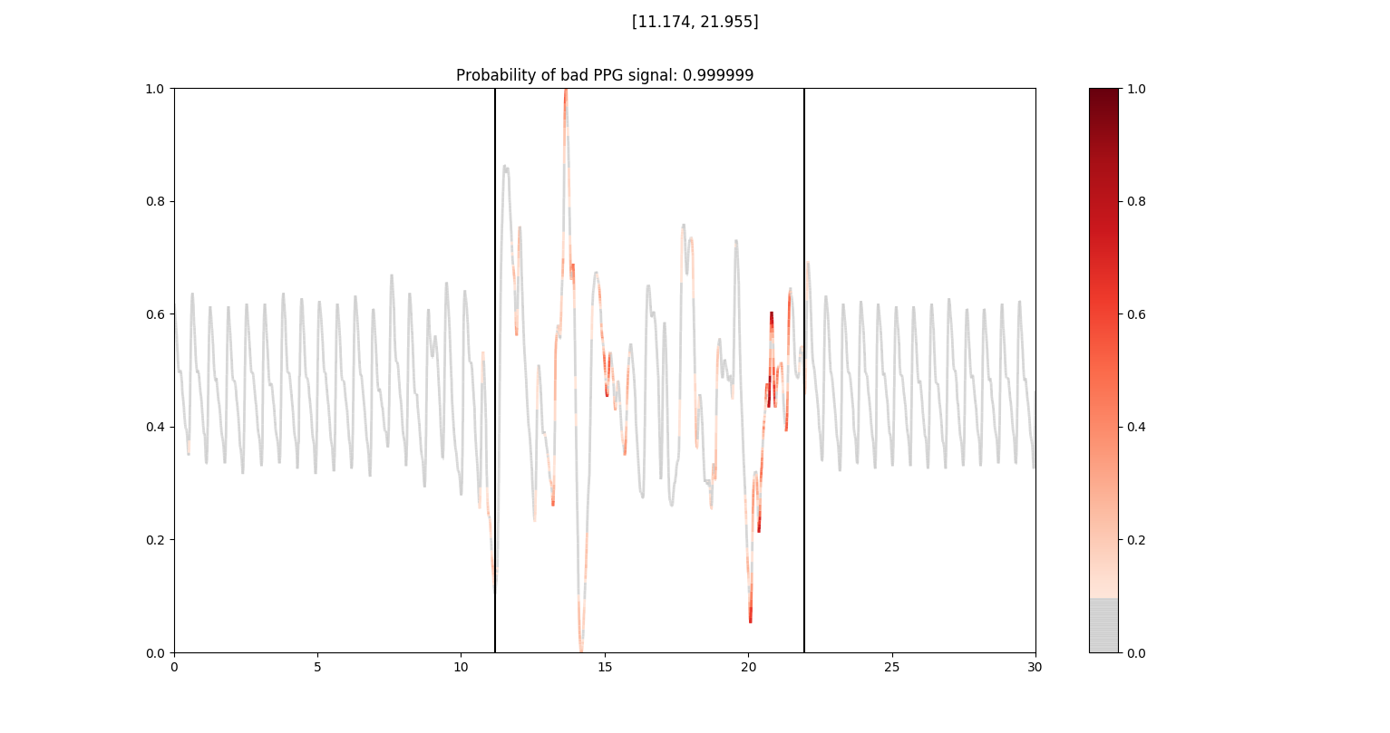
Above: Highlighted are the pixels which the resnet_ppg model associates with a bad ppg. We use guided saliency as our visualization method.

Currently the tools accepts 9 arguments. The tool can also display and visualize both 1D and 2D convolutional neural networks.

--model (str): path to neural network --unprocessed_img(str): path to unprocessed image. (jpg if 2d, npy if 1d) --preprocessed_img (str): path to preprocessed img (Must be npy) --vis (str): Determines visualization type. Either 'cam' (heatmap), 'shap', 'integrated_grad', or 'saliency'

--background (str): Used if you chose 'integrated_grad' or 'shap'. Path to the "background image" (If unsure what "background image" to use, see note below) --conv_layer (int): Used if you chose 'cam'. The index of the last conv2d layer in the model.

--show (bool): Whether to show the image or just save it. --contrast (int): Used for gradient methods ('shap', 'integrated_grad', 'saliency'). A number between 1 to 5, the higher it is, the more gradients are visible. (More info below) --clip (int): Used for gradient methods. A number between 1 to 5, clips the highest gradient to max/clip, so other gradients are visible. --neuron (int): Which neuron in the last layer to visualize. If left blank, the code will visualize the neuron (in the last layer) with the highest activation.

--conv_layer only comes into play if you're using cam and your last pooling layer is GlobalAveragPooling. This is the case for ResNet (1D and 2D) but not VGG.

--background only is necessary for shap or integrated_grad. Basically, these methods require a base image to compare against. This 'base image' should be an image which the model is uncertain about. (For resnet_ppg, you can have a white background, but be sure to preprocess it first. Furthermore, for resnet_ppg_1d, a flatlined data would be at 0.5, so the background should be a flatline of 0.5. These images are at images_2d/background.npy and images_1d/half.npy respectively.

--contrast works by modifying the colormap when displaying gradients. This means that when contrast isn't one, the colormap isn't a linear mapping.

My code is built upon the keras-vis library, the shap library, and the Integrated-Gradients library.

keras vis: https://github.com/raghakot/keras-vis
shap: https://github.com/slundberg/shap
Integrated-Gradients: https://github.com/ankurtaly/Integrated-Gradients

Saliency is implemented by keras-vis and comes from the papers:

1. https://arxiv.org/abs/1312.6034 (vanilla saliency)
2. https://arxiv.org/abs/1412.6806 (discusses guided saliency p.7)

CAM is implemented by keras-vis and comes from the papers:

1. https://arxiv.org/abs/1512.04150 (basic CAM with limited use case.)
2. https://arxiv.org/abs/1610.02391 (generalization of CAM)

Shap is implemented by the shap library and comes from the papers:

(Note: Shap is actually a unified framework of different visualization methods. I'm actually using DeepSHAP, a small part of the framework adapted from DeepLIFT.)

1. https://arxiv.org/abs/1704.02685 (DeepLIFT, the origins of DeepSHAP.)
2. https://arxiv.org/abs/1705.07874 (shap paper containing DeepSHAP.)

integrated_grad is implemented by the Integrated-Gradients library and comes from the paper: (Note that installing Integrated-Gradients isn't necessary; I've copied and pasted a function over from the library instead.)

1. https://arxiv.org/abs/1703.01365

numpy 1.16.4
matplotlib 3.1.0
keras 2.2.4
keras-vis 0.4.1
shap 0.29.2

I used the Signal Quality Index csv and the 1D_model_and_data handed to me by Cheng and Tania. I have the code to process the csv already in the validation_over_images.py file, so if that's what you have, you can just plug and play.

If not, then you want to preprocess your dataset/human annotations yourself and call the visualize_over_dataset function.

Preprocesses the Signal Quality Index csv, but more importantly visualizes the model's attention over all images in visualize_over_dataset function. Can be called as a script or imported as a function.

Saves the visualization so that you can either calculate the ROC metrics using validation_metrics.py or congruence using congruence.py

Analyzes the dataset visualization using one of three metrics. Pixel classification, sectional classification, or interval classification.

Pixel classification attempt to use the model's attention to predict whether the specific pixel is within the human annotated region.

Sectional classification takes the maximum model attention over a section to predict whether the section is human annotated as artifact or clean. (Here the sections are defined by the human annotations. The regions within the human annotations are artifactual sections, whereas the regions outside the human annotations are clean sections.

Interval classification takes the maximum model attention over a fixed interval to predict whether the interval has any artifact within it. Currently the function is hardcoded to break the 7201 length 1d example into 6 5-second segments of 1200 datapoints each. If the interval has any overlap with the human annotations, then its marked as artifactual. Only if it is completely clean then it is marked as clean.

Notes:

1. When I write "we use the model's attention to predict ..." this means that the model attention is thresholded and those are our predictions.
2. Sectional classification vs. Interval classification: The regions within Sectional classification is solely determined by the human annotations, whereas the intervals in interval classification are fixed at 5 seconds.