A Python package for conducting 3D traction force microscopy on multicellular aggregates (so-called spheroids). jointforces provides high-level interfaces to the open-source finite element mesh generator Gmsh and to the Python port of the network optimizer SAENO, facilitating material simulations of contracting multicellular aggregates in highly non-linear biopolymer gels such as collagen. Additionally, jointforces provides an easy-to-use API for analyzing time-lapse images of contracting multicellular aggregates using the particle image velocimetry framework OpenPIV.

Read the article for more information.

Simply install the jointforces via Pip by running following command in the console:

pip install jointforces

Alternatively: The current version of this package can be downloaded as a zip file here, or by cloning this repository. After unzipping, run the following command within the unzipped folder: pip install -e .. This will automatically download and install all other required packages.

jointforces provides example data and pre-computed material simulations for 1.2mg/ml collagen gels as described in Steinwachs et al. (2016). The following code snippet...

• loads a series of images
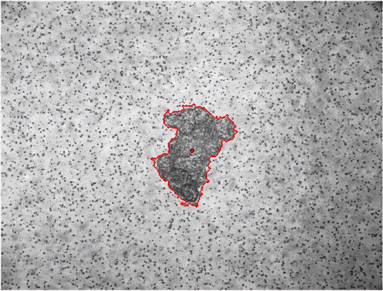
• segments the spheroid in each image
• applies particle image velocimetry to each pair of subsequent images
• compares the resulting matrix deformations to a range of material simulations
• computes the contractile pressure and overall contractility of the spheroid over time

import jointforces as jf

jf.piv.compute_displacement_series('MCF7-time-lapse',  # image folder
                                   '*.tif',            # file pattern
                                   'MCF7-piv',         # output folder
                                   window_size=40,     # PIV window
                                   cutoff=650)         # PIV cutoff

jf.force.reconstruct('MCF7-piv',        # PIV output folder
                     'collagen12.npy',  # lookup table
                     1.29,              # pixel size (µm)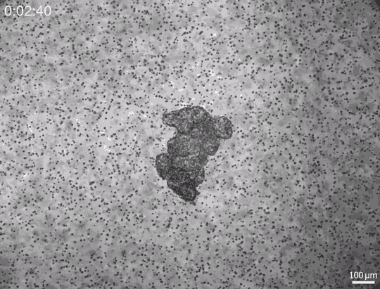
                     'results.xlsx')    # output file

This section details a complete walk-through of the analysis of a 3D traction force microscopy experiment. The data we use in this example can be downloaded here. The data consists of 145 consecutive images of a MCF7 tumor spheroid contracting for 12h within a 1.2mg/ml collagen gel. The contractility of a multicellular aggregate is estimated by comparing the measured deformation field induced by the contracting cells to a set of simulated deformation fields of varying contractility. While we provide precompiled simulations for various materials, this documentation not only covers the force reconstruction step, but also the material simulations.

The module is imported in Python as:

import jointforces as jf

Here, we create a spherical bulk of material (with a radius r_outer=1cm, emulating the biopolymer network) with a small, centered spherical inclusion (with a radius r_inner=100µm, emulating the multicellular aggregate). The keyword-argument length_factor determines the mesh granularity:

jf.mesh.spherical_inclusion('spherical-inclusion.msh', 
                            r_inner=100, 
                            r_outer=10000, 
                            length_factor=0.05)

The resulting mesh is saved as spherical-inclusion.msh and can be displayed in Gmsh using the following command:

jf.mesh.show_mesh('spherical-inclusion.msh')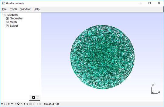

Having created the mesh geometry, we define appropriate boundary conditions and material parameters to emulate the contracting multicellular aggregate in silico. Here, we assume a constant in-bound pressure on the surface of the spherical inclusion (emulating the cells pulling on the surrounding matrix), and no material displacements on the outer boundary of the bulk material (emulating a hard boundary such a the walls of a Petri dish). The goal of the simulation is to obtain the displacements in the surrounding material that are the effect of the pressure exerted by the multicellular aggregate. The following command executes a simulation assuming a pressure of 100Pa and 1.2mg/ml collagen matrix as described in Steinwachs et al. (2016). After successful optimization, the results are stored in the output folder simu:

jf.simulation.spherical_contraction_solver('test.msh', 'simu', pressure=100, material=jf.materials.collagen12)

More detailed information about the output files of a simulation can be found the documentation of the saenopy project.

jointforces provides "pre-configured" material types for collagen gels of three different concentrations (0.6, 1.2, and 2.4mg/ml). Detailed protocols for reproducing these gels can be found in Steinwachs et al. (2016) and Condor et al. (2017). Furthermore, one can define a linear elastic material with a specified stiffness (in Pa) with:

jf.materials.linear(stiffness)

To define a non-linear elastic material, use the custom material type:

jf.materials.custom(K_0, D_0, L_S, D_S)

Non-linear materials are characterized by four parameters:

• K_0: the linear stiffness (in Pa)
• D_0: the rate of stiffness variation during fiber buckling
• L_S: the onset strain for strain stiffening
• D_S: the rate of stiffness variation during strain stiffening A full description of the non-linear material model and the parameters can be found in Steinwachs et al. (2016)

To be able to estimate the contractility of a multicellular aggregate by relating the measured deformation field to simulated ones, we need to execute a set of simulations that cover a wide range of contractile pressures. To speed up this process, jointforces provides a parallelization method that distributes individual instances of the SAENO optimizer across different CPU cores. The following code snippet runs 150 simulations ranging from pressure values of 0.1Pa to 10000Pa (logarithmically spaced):

if __name__ == '__main__':
  jf.simulation.distribute_solver('jf.simulation.spherical_contraction_solver',
                                  const_args={'meshfile': 'spherical-contraction.msh', 'outfolder': 'out_folder',
                                  'material': jf.materials.collagen12},
                                  var_arg='pressure', start=0.1, end=10000, n=150, log_scaling=True, n_cores=2)

The method automatically creates subfolders within the output-folder simu, called simulation000000, simulation000001, and so on, plus a file pressure-values.txt that contains the list of pressure values used in the simulations.

To compare a measured deformation field to a set of simulated ones, we need to create a lookup table that output the expected pressure for a given strain at a given distance from the spheroid (or the expected strain for a given pressure at a given distance). We convert the 3D displacement fields into a set of radial displacement curves and save our material specific lookup-table:

lookup_table = jf.simulation.create_lookup_table_solver(out_folder, x0=1, x1=50, n=100)  
jf.simulation.save_lookup_table(lookup_table,"my_lookup_table.npy")

We can use it to interpolate between individual simulations to create lookup functions for pressure values and strain values:

get_displacement, get_pressure = jf.simulation.load_lookup_functions("my_lookup_table.npy")

For example, we may now ask for the estimated pressure of a spheroid with radius r that induces a deformation of 0.2*r at a distance of 2*r:

print(get_pressure(2, 0.2))
>>> 99.81708381387853

In brief, we can create a custom material lookup table by following the code below. Here, instead of creating an individual mesh, we simply use the provided mesh file here (with r_inner=100, r_outer=10000; in this case we do not need to call the function jf.mesh.spherical_inclusion).

import jointforces as jf

if __name__ == '__main__':
  
    meshfile_loc = r'C:\Users\spherical-inclusion.msh'
    out_folder =   r'C:\Users\lookup_example_folder'
    out_table =   r'C:\Users\lookup_table.npy'
   
    #### your material parameters  (here from a collagen 1.2mg/ml Batch)
    K_0, D_0, L_S, D_S  = 1449 , 0.00215, 0.032, 0.055 
     
    jf.simulation.distribute_solver(  'jf.simulation.spherical_contraction_solver',  
                              const_args={'meshfile': meshfile_loc,     # path to the provided or the new generated mesh
                                          'outfolder': out_folder,    # output folder to store individual simulations
                                          'max_iter': 600,   # maximal iterationts for convergence
                                          'step': 0.0033,  # step size of iteration 
                                          'material': jf.materials.custom(K_0, D_0, L_S, D_S) },      # Enter your own material parameters here
                                          var_arg='pressure', start=0.1, end=1000, n=150, log_scaling=True, n_cores=2, get_initial=True)
       
    lookup_table = jf.simulation.create_lookup_table_solver(out_folder, x0=1, x1=50, n=100)    # output folder for combining the individual simulations
    jf.simulation.save_lookup_table(lookup_table,out_table)

The material lookup-tables can be visualized by using the following function. The shown material was simulated up to 10.000 Pa and we visualize the relative matrix deformations within exactly this pressure range for distances from 2 to 50 spheroid radii (distance and deformation both relative to spheroid size).

jf.simulation.plot_lookup_table("lookup_table.npy", pressure=[0,10000], distance=[2,50])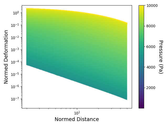

Analog to the following code, the raw data can be plotted into the material lookup-table and thus directly compared to simulations of different times. Each dot corresponds to a single measured deformation around the spheroid at a certain timepoint. The assigned simulation is displayed with dashed lines. A list of timesteps and the paths to the lookup-table and to the evaluated folder (containing u.npy, v.npy and result.xlsx data after piv and force reconstruction) must be given.

jf.simulation.plot_lookup_table(lookup_table=r"lookup_table.npy", pressure=[0,10000],distance=[2,50])  

jf.simulation.plot_lookup_data(r"lookup_table.npy",  # path to lookuptable 
              data_folder = r"pos01_eval", # path to result folder after piv&force-reconstuction containing result.xlsx and piv output
              color_list=["C0","C1","C2","C3","C4"],           # colors for the different times
              timesteps=[2,6, 12*1,12*3,12*20],                # timesteps to plot
              label_list=["10min","30min","1h","3h","20h"])    # corresponding label  (here 1 timestep equals 5 minutes)

plt.ylim(5e-4,6);plt.xlim(1.99,11.5)                           # Zoom to a appropriate range and label the axis  
plt.yticks([1e-3,1e-2,1e-1,1e0],["0.1%","1%","10%","100%"])
plt.xticks([2,3,4,5,6,7,8,9,10],[2,3,4,5,6,7,8,9,10])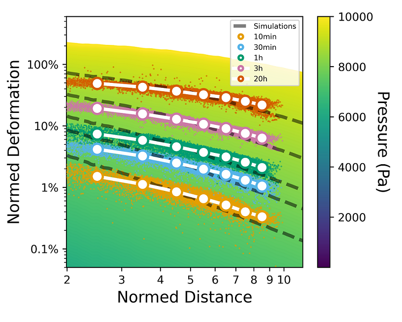

We provide pre-computed lookup-table for different collagen concentrations and further hydrogels gels here. For individual nonlinear materials, the material properties can be determined by using saenopy and can then be used to create a new lookup table. Lookup tables for arbitrary linear elastic material of different stiffness can be easily created using an interpolation function as follows:

jf.simulation.linear_lookup_interpolator(emodulus=250, output_newtable="linear-lookup-emodul-250Pa.pkl")

Up to this point, we have only covered material simulations, but not the analysis of measured time-lapse image series. To detect deformations in the material surrounding the spheroid, jointforces uses the Particle Image Velocimetry algorithm of the OpenPIV package. The following command automatically reads in all image files that match a filterstring within a given folder, and computes the deformation fields between subsequent images, and saves overlay plots of the deformation fields. The exemplary data used in this example can be downloaded here.

jf.piv.compute_displacement_series('MCF7-time-lapse', '*.tif', 'MCF7-piv', 
                                   window_size=40, cutoff=650, draw_mask='False')

The command performs PIV on all *.tif files in the the folder MCF7-time-lapse, the results are saved int he folder MCF7-piv. The window size of the PIV algorithm should be chosen as small as possible to increase spatial resolution, but also large enough to contain multiple fiducial markers for an accurate detection of local material deformations. The cutoff parameter can be used to disregard all displacements that are detected further away from the center than the set value (e.g. because an optical coupler is visible in the corners of the image). With the draw_mask option the user can decide to draw a poylgon mask by hand instead of using the automatic segmentation.

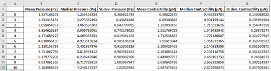
Finally, we may use the lookup functions we have created above and use them to assign the best-fit pressure to each time step of the image series. Additionally, the user supplies the size of one pixel in the image in micrometers. With this information, the surface are of the spheroid is calculated to obtain the total contractility. The output is a Pandas Dataframe containing mean values, median values and standard deviation of both pressure and contractility. If a filename is provided, the results are also saved as an Excel file:

res = jf.force.reconstruct('MCF7-piv', "lookup_table.npy", 6.45/5, 'MCF7-recon.xlsx')

t = np.arange(len(res))*5/60
mu = res['Mean Contractility (µN)']
std = res['St.dev. Contractility (µN)']

plt.figure(figsize=(6, 3))
plt.plot(t, mu, lw=2, c='C0')
plt.fill_between(t, mu-std, mu+std, facecolor='C0', lw=0, alpha=0.5)
plt.grid()
plt.xlabel('Time (h)')
plt.ylabel('Contractility (µN)')
plt.tight_layout()
plt.show()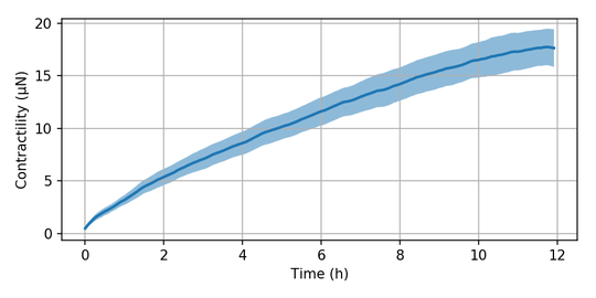

As an alternative to the automatic threshold segmentation manual segmentation can be done using jf.piv.displacement_series(draw_mask=True). Within a pop-up window the borders of the mask can be defined by using left-clicks. When you defined the region of interest you can finish with a right-click and the analysis will continue using the defined mask.

In addition to the total pressure, the pressure within individual angle-sections can be analyzed. The Results.xlsx returns the global Pressure/Force-Values, where we consider all matrix-deformations for the analysis. In the Results_angles.xlsx we divide the matrix into 5-degree angle sections around the center and then calculate the individual Pressure/Values-Values only from the matrix-deformations within these angle-sections. These values might be visualized by using the jf.force.angle_analysis(angle_legend=True)

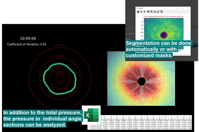
Issue: The angle-sections are by default chosen to 5 degree. Depending on the chosen window-size and image-data the amount of "arrows" in each section may be small. By default we neglect displacements that are in close proximity to the mask or differ highly from the center-axis (to neglect e.g. influence of bubbles). Therefore, it can happen that one might end up with empty angle sections. In that case, you might want to disable the mentioned filters by using the following arguments during force-reconstruction jf.force.reconstruct(r_min = 0, angle_filter = None). Also reducing the windowsize for the angle-analysis could help.

jointforces is tested on Python 3.7 and a Windows 10 64bit system. It depends on numpy, pandas, matplotlib, scipy, scikit-image, openpiv, tqdm, natsort, and dill. We recommend using the Anaconda distribution of Python. Windows users may also take advantage of pre-compiled binaries for all dependencies, which can be found at Christoph Gohlke's page.

The jointforces package itself is licensed under the MIT License. The exemplary data are provided "as is", without any warranty of any kind, express or implied, including but not limited to the warranties of merchantability, fitness for a particular purpose and noninfringement.