


Designed to be a tidy API wrapper for the Bureau of Labor Statistics (BLS.) The package has additional functions to help parse, analyze and visualize the data. The package utilizes "tidyverse" concepts for internal functionality and encourages the use of those concepts with the output data.
- Stable version from CRAN:
install.packages("blscrapeR")- The latest development version from GitHub:
devtools::install_github("keberwein/blscrapeR")Before getting started, you’ll probably want to head over to the BLS and get set up with an API key. While an API key is not required to use the package, the query limits are much higher if you have a key and you’ll have access to more data. Plus, it’s free (as in beer), so why not?
For “quick and dirty” type of analysis, the package has some quick functions that will pull metrics from the API without series numbers. These quick functions include unemployment, employment, and civilian labor force on a national level.
library(blscrapeR)
# Grab the Unemployment Rate (U-3)
df <- quick_unemp_rate()
head(df, 5)
#> # A tibble: 5 x 6
#>    year    period periodName value footnotes  seriesID
#>   <dbl>    <list>     <list> <dbl>    <list>    <list>
#> 1  2017 <chr [1]>  <chr [1]>   4.1 <chr [1]> <chr [1]>
#> 2  2017 <chr [1]>  <chr [1]>   4.2 <chr [1]> <chr [1]>
#> 3  2017 <chr [1]>  <chr [1]>   4.4 <chr [1]> <chr [1]>
#> 4  2017 <chr [1]>  <chr [1]>   4.3 <chr [1]> <chr [1]>
#> 5 2017 <chr [1]> <chr [1]> 4.4 <chr [1]> <chr [1]>Some knowledge of BLS ids are needed to query the API. The package includes a "fuzzy search" function to help find these ids. There are currently more than 75,000 series ids in the package's internal data set, series_ids. While these aren't all the series ids the BLS offers, it contains the most popular. The BLS Data Finder is another good resource for finding series ids, that may not be in the internal data set.
library(blscrapeR)
# Find series ids relating to the total labor force in LA.
ids <- search_ids(keyword = c("Labor Force", "Los Angeles"))
head(ids)
#> # A tibble: 6 x 4
#>                                                                  series_title
#>                                                                         <chr>
#> 1 Labor Force: Balance Of California, State Less Los Angeles-Long Beach-Glend
#> 2  Labor Force: Los Angeles-Long Beach-Glendale, Ca Metropolitan Division (S)
#> 3 Labor Force: Balance Of California, State Less Los Angeles-Long Beach-Glend
#> 4       Labor Force: Los Angeles-Long Beach, Ca Combined Statistical Area (U)
#> 5                                     Labor Force: Los Angeles County, Ca (U)
#> 6                                       Labor Force: Los Angeles City, Ca (U)
#> # ... with 3 more variables: series_id <chr>, seasonal <chr>,
#> # periodicity_code <chr>library(blscrapeR)
# Find series ids relating to median weekly earnings of women software developers.
ids <- search_ids(keyword = c("Earnings", "Software", "Women"))
head(ids)
#> # A tibble: 1 x 4
#> series_title
#> <chr>
#> 1 (Unadj)- Median Usual Weekly Earnings (Second Quartile), Employed Full Time
#> # ... with 3 more variables: series_id <chr>, seasonal <chr>,
#> # periodicity_code <chr>You should consider getting an API key form the BLS. The package has a function to install your key in your .Renviron so you’ll only have to worry about it once. Plus, it will add extra security by not having your key hard-coded in your scripts for all the world to see.
| Service | Version 2.0 (Registered) | Version 1.0 (Unregistered) |
|---|---|---|
| Daily query limit | 500 | 25 |
| Series per query limit | 50 | 25 |
| Years per query limit | 20 | 10 |
| Net/Percent Changes | Yes | No |
| Optional annual averages | Yes | No |
| Series descriptions | Yes | No |
library(blscrapeR)
set_bls_key("YOUR_KEY_IN_QUOTATIONS")
# First time, reload your enviornment so you can use the key without restarting R.
readRenviron("~/.Renviron")
# You can check it with:
Sys.getenv("BLS_KEY")
Note: The above script will add a line to your .Renviron file to be re-used when ever you are in the package. If you are not comfortable with that, you can add the following line to your .Renviron file manually to produce the same result.
BLS_KEY='YOUR_KEY_IN_SINGLE_QUOTES'
Now that you have an API key installed, you can call your key in the package’s function arguments with "BLS_KEY". Don't forget the quotes! If you just HAVE to have your key hard-coded in your scripts, you can also pass they key as a string.
library(blscrapeR)

# Grab several data sets from the BLS at onece.
# NOTE on series IDs:
# EMPLOYMENT LEVEL - Civilian labor force - LNS12000000
# UNEMPLOYMENT LEVEL - Civilian labor force - LNS13000000
# UNEMPLOYMENT RATE - Civilian labor force - LNS14000000
df <- bls_api(c("LNS12000000", "LNS13000000", "LNS14000000"),
              startyear = 2008, endyear = 2017, Sys.getenv("BLS_KEY")) %>%
    # Add time-series dates
    dateCast()
# Plot employment level
library(ggplot2)
gg1200 <- subset(df, seriesID=="LNS12000000")
library(ggplot2)
ggplot(gg1200, aes(x=date, y=value)) +
geom_line() +
labs(title = "Employment Level - Civ. Labor Force")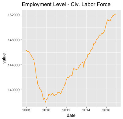
library(blscrapeR)
library(tidyverse)
# Median Usual Weekly Earnings by Occupation, Unadjusted Second Quartile.
# In current dollars
df <- bls_api(c("LEU0254530800", "LEU0254530600"), startyear = 2000, endyear = 2016, registrationKey = Sys.getenv("BLS_KEY")) %>%
    spread(seriesID, value) %>% dateCast()
# A little help from ggplot2!
library(ggplot2)
ggplot(data = df, aes(x = date)) +
geom_line(aes(y = LEU0254530800, color = "Database Admins.")) +
geom_line(aes(y = LEU0254530600, color = "Software Devs.")) +
labs(title = "Median Weekly Earnings by Occupation") + ylab("value") +
theme(legend.position="top", plot.title = element_text(hjust = 0.5)) 
For more advanced usage, please see the package vignettes.
Like the the “quick functions” for requesting API data, there are two "quick" map functions, bls_map_county() and bls_map_state(). These functions are designed to work with two helper functions get_bls_county() and get get_bls_state(). Each helper function downloads recent data for unemployment rate, unemployment level, employment rate, employment level and civilian labor force. These functions do not pull data from the API, rather they pull data from text files and do not count against daily query limits.
Note: Even though the get_bls functions return data in the correct formats, the bls_map functions can be used with any data set that includes FIPS codes.
The example below maps the current unemployment rate by county. Alaska and Hawaii have to re-located to save space.
library(blscrapeR)
# Grap the data in a pre-formatted data frame.
# If no argument is passed to the function it will load the most recent month's data.
df <- get_bls_county()

#Use map function with arguments.
map_bls(map_data = df, fill_rate = "unemployed_rate",
               labtitle = "Unemployment Rate by County")
What's R mapping without some interactivity? Below we’re using two additional packages, leaflet, which is popular for creating interactive maps and tigris, which allows us to download the exact shape files we need for these data and includes a few other nice tools.
# Leaflet map
library(blscrapeR)
library(tigris)
library(leaflet)
map.shape <- counties(cb = TRUE, year = 2015)
df <- get_bls_county()

# Slice the df down to only the variables we need and rename "fips" colunm
# so I can get a cleaner merge later.
df <- df[, c("unemployed_rate", "fips")]
colnames(df) <- c("unemployed_rate", "GEOID")

# Merge df with spatial object.
leafmap <- geo_join(map.shape, df, by="GEOID")

# Format popup data for leaflet map.
popup_dat <- paste0("<strong>County: </strong>",
                    leafmap$NAME,
                    "<br><strong>Value: </strong>",
                    leafmap$unemployed_rate)

pal <- colorQuantile("YlOrRd", NULL, n = 20)
# Render final map in leaflet.
leaflet(data = leafmap) %>% addTiles() %>%
    addPolygons(fillColor = ~pal(unemployed_rate),
                fillOpacity = 0.8,
                color = "#BDBDC3",
                weight = 1,
                popup = popup_dat)
Note: This is just a static image since the full map would not be as portable for the purpose of documentation.


