本文用Python实现了BP神经网络分类算法,根据鸢尾花的4个特征,实现3种鸢尾花的分类。 算法参考文章:纯Python实现鸢尾属植物数据集神经网络模型
iris_data_classification_bpnn_V1.py 需使用 bpnn_V1数据集 文件夹中的数据
iris_data_classification_bpnn_V2.py 需使用 bpnn_V2数据集 文件夹中的数据
iris_data_classification_knn.py 需使用 原始数据集 文件夹中的数据
iris_data_cluster_sklearn.py 需使用 sklearn数据集 文件夹中的数据
不同数据集里数据都是一样的,只是为了程序使用方便而做了一些格式的变动。
2020.07.21更新: 增加了分类结果可视化result_visualization。
2020.07.09更新: 完善代码中取数据部分的操作。
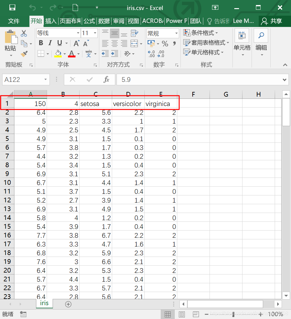
鸢尾花数据集包含4种特征,萼片长度(Sepal Length)、萼片宽度(Sepal Width)、花瓣长度(Petal Length)和花瓣宽度(Petal Width),以及3种鸢尾花Versicolor、Virginica和Setosa。
数据集共151行,5列:
- 第1行是数据说明,“150”表示共150条数据;“4”表示特征数;“setosa、versicolor、virginica”是三类花的名字
- 第2行至第151行是150条数据
- 第1至4列是Sepal Length、Sepal Width、Petal Length、Petal Width 4个特征
- 第5列是花的类别,用0、1、2表示
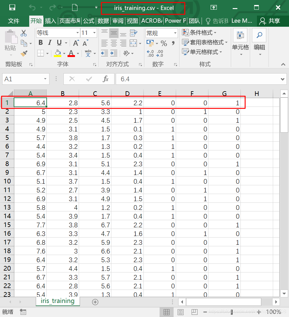
为方便起见,需要对数据集稍作处理:
- 将150条数据分隔为两个文件,前120条另存为
iris_training.csv,即训练集;后30条另存为iris_test.csv,即测试集; - 训练集和测试集都删去第1行;
- 训练集和测试集都删去原来的最后1列,并新增加3列,目的是用3列来表示鸢尾花的分类:如果原来最后一列是0,则新增加的3列为(0,0,0);如果原来最后一列是1,则新增加的3列为(0,1,0);如果原来最后一列是2,则新增加的3列为(0,0,1)。
纯Python实现鸢尾属植物数据集神经网络模型 这篇文章中讲解得更为详细。本人对代码做了略微的修改,并增加了评估模型准确率的predict()函数。
以下代码对应的是iris_data_classification_bpnn_V2.py文件
import pandas as pd
import numpy as np
import datetime
import matplotlib.pyplot as plt
from pandas.plotting import radviz
'''
    构建一个具有1个隐藏层的神经网络,隐层的大小为10
    输入层为4个特征,输出层为3个分类
    (1,0,0)为第一类,(0,1,0)为第二类,(0,0,1)为第三类
'''


# 1.初始化参数
def initialize_parameters(n_x, n_h, n_y):
    np.random.seed(2)

    # 权重和偏置矩阵
    w1 = np.random.randn(n_h, n_x) * 0.01
    b1 = np.zeros(shape=(n_h, 1))
    w2 = np.random.randn(n_y, n_h) * 0.01
    b2 = np.zeros(shape=(n_y, 1))

    # 通过字典存储参数
    parameters = {'w1': w1, 'b1': b1, 'w2': w2, 'b2': b2}

    return parameters


# 2.前向传播
def forward_propagation(X, parameters):
    w1 = parameters['w1']
    b1 = parameters['b1']
    w2 = parameters['w2']
    b2 = parameters['b2']

    # 通过前向传播来计算a2
    z1 = np.dot(w1, X) + b1     # 这个地方需注意矩阵加法:虽然(w1*X)和b1的维度不同,但可以相加
    a1 = np.tanh(z1)            # 使用tanh作为第一层的激活函数
    z2 = np.dot(w2, a1) + b2
    a2 = 1 / (1 + np.exp(-z2))  # 使用sigmoid作为第二层的激活函数

    # 通过字典存储参数
    cache = {'z1': z1, 'a1': a1, 'z2': z2, 'a2': a2}

    return a2, cache


# 3.计算代价函数
def compute_cost(a2, Y, parameters):
    m = Y.shape[1]      # Y的列数即为总的样本数

    # 采用交叉熵(cross-entropy)作为代价函数
    logprobs = np.multiply(np.log(a2), Y) + np.multiply((1 - Y), np.log(1 - a2))
    cost = - np.sum(logprobs) / m

    return cost


# 4.反向传播(计算代价函数的导数)
def backward_propagation(parameters, cache, X, Y):
    m = Y.shape[1]

    w2 = parameters['w2']

    a1 = cache['a1']
    a2 = cache['a2']

    # 反向传播,计算dw1、db1、dw2、db2
    dz2 = a2 - Y
    dw2 = (1 / m) * np.dot(dz2, a1.T)
    db2 = (1 / m) * np.sum(dz2, axis=1, keepdims=True)
    dz1 = np.multiply(np.dot(w2.T, dz2), 1 - np.power(a1, 2))
    dw1 = (1 / m) * np.dot(dz1, X.T)
    db1 = (1 / m) * np.sum(dz1, axis=1, keepdims=True)

    grads = {'dw1': dw1, 'db1': db1, 'dw2': dw2, 'db2': db2}

    return grads


# 5.更新参数
def update_parameters(parameters, grads, learning_rate=0.4):
    w1 = parameters['w1']
    b1 = parameters['b1']
    w2 = parameters['w2']
    b2 = parameters['b2']

    dw1 = grads['dw1']
    db1 = grads['db1']
    dw2 = grads['dw2']
    db2 = grads['db2']

    # 更新参数
    w1 = w1 - dw1 * learning_rate
    b1 = b1 - db1 * learning_rate
    w2 = w2 - dw2 * learning_rate
    b2 = b2 - db2 * learning_rate

    parameters = {'w1': w1, 'b1': b1, 'w2': w2, 'b2': b2}

    return parameters


# 6.模型评估
def predict(parameters, x_test, y_test):
    w1 = parameters['w1']
    b1 = parameters['b1']
    w2 = parameters['w2']
    b2 = parameters['b2']

    z1 = np.dot(w1, x_test) + b1
    a1 = np.tanh(z1)
    z2 = np.dot(w2, a1) + b2
    a2 = 1 / (1 + np.exp(-z2))

    # 结果的维度
    n_rows = y_test.shape[0]
    n_cols = y_test.shape[1]

    # 预测值结果存储
    output = np.empty(shape=(n_rows, n_cols), dtype=int)

    for i in range(n_rows):
        for j in range(n_cols):
            if a2[i][j] > 0.5:
                output[i][j] = 1
            else:
                output[i][j] = 0

    print('预测结果:')
    print(output)
    print('真实结果:')
    print(y_test)

    count = 0
    for k in range(0, n_cols):
        if output[0][k] == y_test[0][k] and output[1][k] == y_test[1][k] and output[2][k] == y_test[2][k]:
            count = count + 1
        else:
            print(k)

    acc = count / int(y_test.shape[1]) * 100
    print('准确率:%.2f%%' % acc)

    return output


# 建立神经网络
def nn_model(X, Y, n_h, n_input, n_output, num_iterations=10000, print_cost=False):
    np.random.seed(3)

    n_x = n_input           # 输入层节点数
    n_y = n_output          # 输出层节点数

    # 1.初始化参数
    parameters = initialize_parameters(n_x, n_h, n_y)

    # 梯度下降循环
    for i in range(0, num_iterations):
        # 2.前向传播
        a2, cache = forward_propagation(X, parameters)
        # 3.计算代价函数
        cost = compute_cost(a2, Y, parameters)
        # 4.反向传播
        grads = backward_propagation(parameters, cache, X, Y)
        # 5.更新参数
        parameters = update_parameters(parameters, grads)

        # 每1000次迭代,输出一次代价函数
        if print_cost and i % 1000 == 0:
            print('迭代第%i次,代价函数为:%f' % (i, cost))

    return parameters


# 结果可视化
# 特征有4个维度,类别有1个维度,一共5个维度,故采用了RadViz图
def result_visualization(x_test, y_test, result):
    cols = y_test.shape[1]
    y = []
    pre = []

    # 反转换类别的独热编码
    for i in range(cols):
        if y_test[0][i] == 0 and y_test[1][i] == 0 and y_test[2][i] == 1:
            y.append('setosa')
        elif y_test[0][i] == 0 and y_test[1][i] == 1 and y_test[2][i] == 0:
            y.append('versicolor')
        elif y_test[0][i] == 1 and y_test[1][i] == 0 and y_test[2][i] == 0:
            y.append('virginica')

    for j in range(cols):
        if result[0][j] == 0 and result[1][j] == 0 and result[2][j] == 1:
            pre.append('setosa')
        elif result[0][j] == 0 and result[1][j] == 1 and result[2][j] == 0:
            pre.append('versicolor')
        elif result[0][j] == 1 and result[1][j] == 0 and result[2][j] == 0:
            pre.append('virginica')
        else:
            pre.append('unknown')

    # 将特征和类别矩阵拼接起来
    real = np.column_stack((x_test.T, y))
    prediction = np.column_stack((x_test.T, pre))

    # 转换成DataFrame类型,并添加columns
    df_real = pd.DataFrame(real, index=None, columns=['Sepal Length', 'Sepal Width', 'Petal Length', 'Petal Width', 'Species'])
    df_prediction = pd.DataFrame(prediction, index=None, columns=['Sepal Length', 'Sepal Width', 'Petal Length', 'Petal Width', 'Species'])

    # 将特征列转换为float类型,否则radviz会报错
    df_real[['Sepal Length', 'Sepal Width', 'Petal Length', 'Petal Width']] = df_real[['Sepal Length', 'Sepal Width', 'Petal Length', 'Petal Width']].astype(float)
    df_prediction[['Sepal Length', 'Sepal Width', 'Petal Length', 'Petal Width']] = df_prediction[['Sepal Length', 'Sepal Width', 'Petal Length', 'Petal Width']].astype(float)

    # 绘图
    plt.figure('真实分类')
    radviz(df_real, 'Species', color=['blue', 'green', 'red', 'yellow'])
    plt.figure('预测分类')
    radviz(df_prediction, 'Species', color=['blue', 'green', 'red', 'yellow'])
    plt.show()


if __name__ == "__main__":
    # 读取数据
    data_set = pd.read_csv('D:\\iris_training.csv', header=None)

    # 第1种取数据方法:
    X = data_set.iloc[:, 0:4].values.T          # 前四列是特征,T表示转置
    Y = data_set.iloc[:, 4:].values.T           # 后三列是标签

    # 第2种取数据方法:
    # X = data_set.ix[:, 0:3].values.T
    # Y = data_set.ix[:, 4:6].values.T

    # 第3种取数据方法:
    # X = data_set.loc[:, 0:3].values.T
    # Y = data_set.loc[:, 4:6].values.T

    # 第4种取数据方法:
    # X = data_set[data_set.columns[0:4]].values.T
    # Y = data_set[data_set.columns[4:7]].values.T
    Y = Y.astype('uint8')

    # 开始训练
    start_time = datetime.datetime.now()
    # 输入4个节点,隐层10个节点,输出3个节点,迭代10000次
    parameters = nn_model(X, Y, n_h=10, n_input=4, n_output=3, num_iterations=10000, print_cost=True)
    end_time = datetime.datetime.now()
    print("用时:" + str((end_time - start_time).seconds) + 's' + str(round((end_time - start_time).microseconds / 1000)) + 'ms')

    # 对模型进行测试
    data_test = pd.read_csv('D:\\iris_test.csv', header=None)
    x_test = data_test.iloc[:, 0:4].values.T
    y_test = data_test.iloc[:, 4:].values.T
    y_test = y_test.astype('uint8')

    result = predict(parameters, x_test, y_test)

    # 分类结果可视化
    result_visualization(x_test, y_test, result)
最终结果:

分类的可视化效果,左侧为测试集的真实分类,右侧为模型的预测分类结果,采用的是RadViz图:
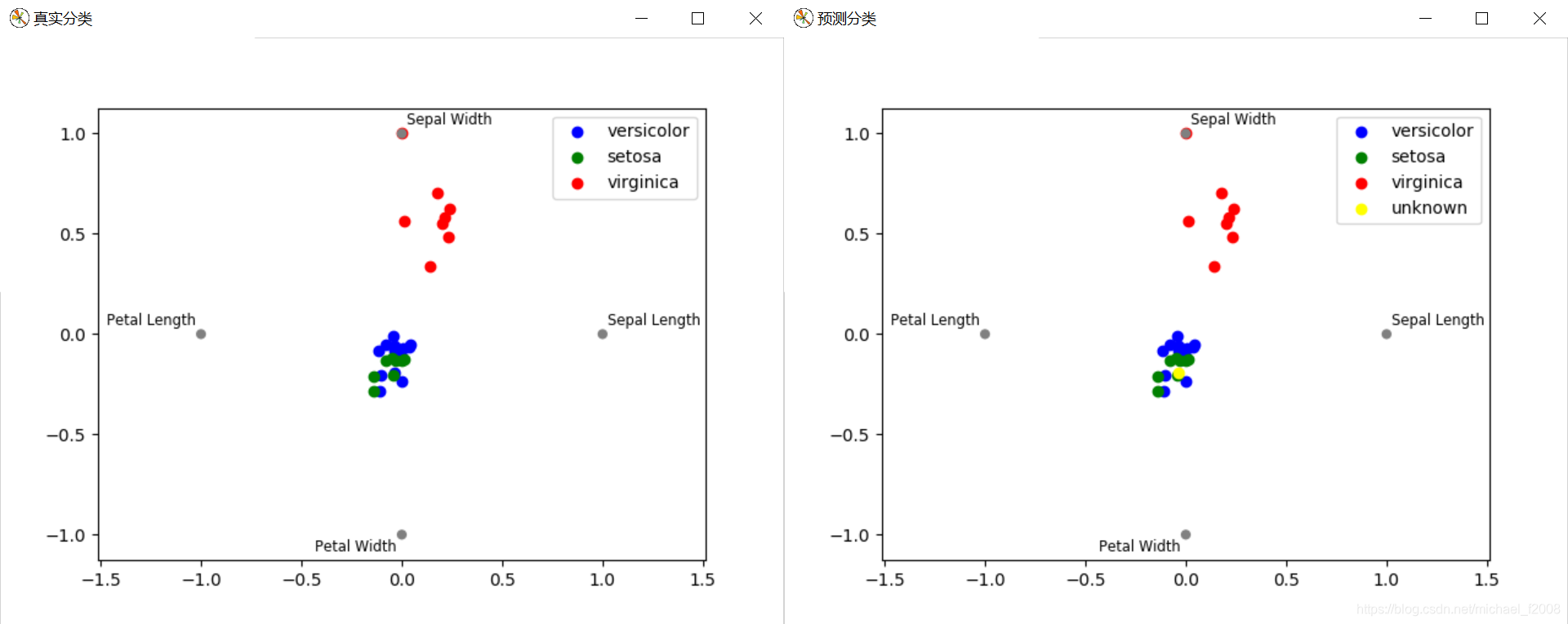
每次运行时准确率可能都不一样,可以通过调整学习率、隐节点数、迭代次数等参数来改善模型的效果。
算法的实现总共分为6步:
- 初始化参数
- 前向传播
- 计算代价函数
- 反向传播
- 更新参数
- 模型评估
