

![]()
Visualization library for Keras Neural Networks
pip3 install kviz
On Fedora
sudo dnf install python3-devel graphviz graphviz-devel
On Ubuntu
sudo apt-get install graphviz graphviz-dev
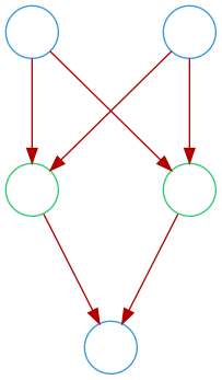
You can visualize the architecture of your keras model as such:
    model = keras.models.Sequential()
    model.add(layers.Dense(2, input_dim=2))
    model.add(layers.Dense(1, activation="sigmoid"))
    model.compile(loss="binary_crossentropy")

    dg = DenseGraph(model)
    dg.render()
Produces the following graph:
You can visualize the learned decision boundary of your model as such:
    model = keras.models.Sequential()
    model.add(layers.Dense(2, input_dim=2, activation='relu'))
    model.add(layers.Dense(1, activation='sigmoid'))
    model.compile(loss="binary_crossentropy")

    # Generate data that looks like 2 concentric circles
    t, _ = datasets.make_blobs(n_samples=200, centers=[[0, 0]], cluster_std=1, random_state=1)
    X = np.array(list(filter(lambda x: x[0]**2 + x[1]**2 < 1 or x[0]**2 + x[1]**2 > 1.5, t)))
    Y = np.array([1 if x[0]**2 + x[1]**2 >= 1 else 0 for x in X])

    dg = DenseGraph(model)
    dg.animate_learning(X, Y, snap_freq=20, duration=300, batch_size=4, epochs=1000, verbose=0)
Which produces the following GIF:

We can try different activation functions, network architectures, etc. to see what works best. For example, from looking at the GIF we can see that the neural net is trying to learn a decision boundary that is a combination of two straight lines. Clearly this is not going to work for a circular decision boundary. We could expect to better approximate this circular decision boundary if we had more straight lines to combine. We could try changing the number of neurons in the hidden layer to 3 or more (to learn higher dimensional features). This produces the following (for 4 hidden neurons):

Instead, we can try changing the activation in the hidden layer to a custom_activation
function that is non-linear and matches our intuition of what circles are:
    def custom_activation(x):
        return x**2

    model = keras.models.Sequential()
    model.add(layers.Dense(2, input_dim=2, activation=custom_activation))
    model.add(layers.Dense(1, activation='sigmoid'))
    model.compile(loss="binary_crossentropy")
which produces:

You can visualize which nodes activate in the network as a function of a set of inputs.
    model = keras.models.Sequential()
    model.add(layers.Dense(2, input_dim=2, activation='sigmoid'))
    model.add(layers.Dense(1, activation='sigmoid'))
    model.compile(loss="binary_crossentropy")

    X = np.array([
        [0,0],
        [0,1],
        [1,0],
        [1,1]])
    Y = np.array([x[0]^x[1] for x in X]) # Xor function

    history = model.fit(X, Y, batch_size=4, epochs=1000, verbose=0)

    dg = DenseGraph(model)
    dg.animate_activations(X)
Produces the following decision boundary (visualized using matplotlib):

And the following GIF:

The darker the node the higher the activation is at that node.
    import sklearn.datasets as datasets

    model = keras.models.Sequential()
    model.add(layers.Dense(3, input_dim=2, activation=ACTIVATION))
    model.add(layers.Dense(1, activation=ACTIVATION))
    model.compile(loss="binary_crossentropy")

    centers = [[.5, .5]]
    t, _ = datasets.make_blobs(n_samples=50, centers=centers, cluster_std=.1)
    X = np.array(t)
    Y = np.array([1 if x[0] - x[1] >= 0 else 0 for x in X])

    history = model.fit(X, Y)

    dg = DenseGraph(model)
    dg.animate_activations(X, duration=.3)
Produces the following decision boundary (visualized using matplotlib):

And the following GIF:
At a glance you can see that the activations of the middle hidden node results in predictions of class 0 while the activation of the left-most and right-most hiddent nodes result in predictions of class 1.
You can modify the node activation graph. The node activation graph consists of a pyplot graph and a networkx graph. You can change the color and marker of the points in the pyplot graph, and attributes like the color and shape of each node in the networkx graph.
For the pyplot graph, you can use parameters x_color and x_marker when
calling render to change the colors and shapes of the points.
For the networkx graph, first, you need to use the get_graph method to get
the networkx graph from DenseGraph. Then, you can modify the graph as needed.
One possible way is to loop through the nodes of the graph and use
set_node_attributes and set_edge_attributes from networkx. Finally, you
can use the set_graph method to pass the modified graph to DenseGraph and
call render to get the visualization.
The index of each node is defined as a string, which equals the index of the layer (starts from 0) plus "_" plus the index of the node in that layer (starts from 0). For example, the index "0_0" means the first node ("0") in the first layer ("0").
We provide a function called unique_index with which you can conveniently
get the index of a certain node. The input to this function is the sequence of the
layer with the node (starts from 0), and the sequence of the node in the layer (also
starts from 0). We suggest you use this function instead of explicitly computing
the index, because in the future we may update the way we represent a node.
The index of an edge is a tuple consisting of 2 nodes that are connected by it. The node in the upper layer usually comes first. For example, ("0_0", "1_0") is the index of an edge that connects node "0_0" and node "1_0".
Below is an example using the XOR function: (assume we already had a keras model; you can get one using the codes above)
    from networkx import set_node_attributes, set_edge_attributes
    from kviz.helper_functions import unique_index

    # "model" is already a trained keras model.
    dg = DenseGraph(model)

    # Get the networkx graph.
    the_graph = dg.get_graph()

    # Loop through the graph by looping through the model.
    for l in range(len(model.layers)):  # get number of layers
        layer = model.layers[l]
        for n in range(0, layer.input_shape[1]):  # get number of nodes in that layer
            set_node_attributes(the_graph, {
                unique_index(l, n): {
                    'shape': "diamond",
                    'color': "#00ff00",
                    'label': ""
                }
            })

            # Here, set the attributes for nodes in the output layer, which is the last
            # layer of this model.
            for h in range(0, layer.output_shape[1]):
                if l == len(model.layers) - 1:  # check if the layer is the last layer
                    set_node_attributes(the_graph, {
                        unique_index(l + 1, h): {
                            'shape': "square",
                            'color': "#ff0000",
                            'label': ""
                        }
                    })
                # Now set the attributes of edges.
                # The index of an edge is an tuple consisting of the indexes of
                # the 2 nodes that are connected by it.
                set_edge_attributes(the_graph, {
                    (unique_index(l ,n), unique_index(l + 1, h)): {
                        'color': "#0000ff"
                    }
                })

    # Pass the modified network graph to DenseGraph.
    dg.set_graph(the_graph)

    # Get the visualization & set the color and marker in the pyplot graph.
    dg.animate_activations(X, x_color="#FF0000", x_marker="^")
Of course, you do not need to loop through the model if you already know the
number of layers and number of nodes in each layer. You can directly set the
attributes of every node by its index using set_node_attributes
and set_edge_attributes.
Below is the code example. It will give the same result as the codes above.
    from networkx import set_node_attributes, set_edge_attributes
    from kviz.helper_functions import unique_index

    dg = DenseGraph(model)

    the_graph = dg.get_graph()

    # the input layer has a shape of 2, same as the inner dense layer
    # set the input nodes first
    l = 0
    for n in range(2):  # a shape of 2
        set_node_attributes(the_graph, {
            unique_index(l, n): {
                'shape': "diamond",
                'color': "#00ff00",
                'label': ""
            }
        })

    # set the inner dense layer then. In this case, there is only 1 inner dense layer.
    l = 1
    for n in range(2):  # a shape of 2
        set_node_attributes(the_graph, {
            unique_index(l, n): {
                'shape': "diamond",
                'color': "#00ff00",
                'label': ""
            }
        })

    # set the output dense layer, which has a shape of 1
    l = 2
    set_node_attributes(the_graph, {
        unique_index(l, 0): {
            'shape': "square",
            'color': "#ff0000",
            'label': ""
        }
    })

    # finally set all the edges:
    # here we have a graph of 3 layers
    # the first 2 layers have a shape of 2, while the last layer has a shape of 1
    # a total of 2 * 2 + 2 * 1 = 6 edges
    # for convenience, all edges are listed below
    edge_ids = [(unique_index(0 ,0), unique_index(1, 0)), (unique_index(0, 1), unique_index(1, 0)),
                (unique_index(0, 0), unique_index(1, 1)), (unique_index(0, 1), unique_index(1, 1)),
                (unique_index(1, 0), unique_index(2, 0)), (unique_index(1, 1), unique_index(2, 0))]

    for edge_id in edge_ids:
        set_edge_attributes(the_graph, {
            edge_id: {
                'color': "#0000ff"
            }
        })

    dg.set_graph(the_graph)
    dg.animate_activations(X, x_color="#FF0000", x_marker="^")
The result is:
Bump the release version in the setup.py file, then run:
    make clean
    make build
    make release


