global-healthy-liveable-cities / global-indicators Goto Github PK

The global indicators software tool was initially designed as a proof of concept spatial indicator analysis workflow for 25 cities. However, to work for an open ended number of cities, a walkability index cannot be calculated based on sub-components scored relative to the observed values across all cities. This would mean all cities walkability scores would require re-calculation as each new city were added. Instead, benchmarking against some fixed target(s) which are ideally policy relevant, could be desirable.

This would be relatively easy to implement, but determining which are the relevant thresholds that could apply as appropriate targets across different cultural, economic and geographic contexts

(not an urgent issue - but one to think about as we polish our code)

While the use of clearly invalid numbers like -999, -777 or -666 as error codes is not unusual, I think it is generally acknowledged as a practice that should be avoided where possible --- particularly when dealing with a numeric estimate.

I think it is a bad idea to store distance estimates as -999, as a logical thing for a new future user of this data to do is evaluate for access less than or equal to some threshold distance of interest (e.g. 500 metres). If someone were to naively do this, they would return all the data, which they may find surprising, but it could lead to misunderstandings or a waste of time as they try to figure out what has happened.

Similarly, when a new user opens the data, and they look to visualise it in QGIS (like I just did) might get sudden warning bells --- "wtf?! negative distances?!!!"

We should save people the stress and cortisol exposure and just make it more easy to not misuse or misvisualise the data.

It would make sense to have those sample points with out access to have a result of nan. This would mean we would have to change our use of dropping nans - but as Shirley has demonstrated, this is problematic too.

We are opening an issue to document, propose, and discuss any prior literature work.

Which articles can help solidify the quality analysis framework for this project?

It would be helpful if everyone can add comments here regarding:

• Discussion and proposal of previous literature work

• Quality assessments of OSM datasets literature

Hey everyone,

David and I have been looking closer into the official datasets from Sao Paulo, Olomouc, and Belfast. Right now, we are trying to 'pair down' the datasets so that we are able to make more 'apples to apples' comparisons between the official and OSM derived datasets.

Sao Paulo:
Sao Paolo's official dataset has 939 destinations (point data) as shown below.

There are category labels, so we were able to sort out the relevant categories of data. After sorting, there are 34 relevant destinations.

Olomouc:
Olomouc's official dataset has 63 destinations (point data) as shown below.

There is no category label, so we are unable to systematically sort thru the data. Looking at it manually, however, it does seem to be that each of the points is a supermarket (we looked at about 10).

We think that means that we can just use all the Olomouc data for the apples to apples comparison.

Belfast:
Belfast's official dataset has 1,479 destinations (polygon data) as shown below.

For Belfast, there is no name or category data, so we are unsure how to sort out food-related destinations that are out of scope (like farmer's markets and restaurants). Does anyone have ideas?

Additionally, should we think of different ways to validate data, considering that it is polygon data instead of point data?

For Coding:
@gboeing On our call on Tuesday, you advised us to make sure that the config files were updated for each city so that the relevant destinations could be extracted. Considering that this can be done for only one of the three cities, should we change our approach?

(not urgent - but something for us to think about as we polish this code into the shape we want it to be)

I think its a bad idea that we modify our input data source files; we should aim to keep a clear distinction what is input and what is output. Even if the layers in the geopackages aren't modified, we shouldn't add outputs to the input. Doing this makes it unclear by looking at files if things have been processed.

A better approach might be to create a time stamped output geopackage, containing only the newly generated output layers.

A naming convention could use a suffix like 'output-yyyy-mm-dd', like:

bangkok_th_2019_1600m_buffer_output-2020-02-28.gpkg

This would allow us to relate our outputs back directly to the date they were first generated (as file system date modified dates aren't always reliable, or standard across systems). So, when we change our code for the in earnest outputs, we can tell at a glance when an output was generated so we can't get them mixed up.

Technically, the csv could be table in the output geopackage if we wanted to keep output resources contained in a single file (since a gpkg file is just an sqlite database); although that would just be a nicety to keep things tidy.

(not urgent - but good to be clear when we write papers)

Currently, the codes appear to implement as
access = (distance < 500)

e.g. when I run these queries, the maximum distance is 499 (after I have cast it as Int64):

>>> np.nanmax(gdf_nodes_poi_dist.sp_nearest_node_supermarket_dist)
499
>>> np.nanmax(gdf_nodes_poi_dist.sp_nearest_node_pt_dist)
499
>>> np.nanmax(gdf_nodes_poi_dist.sp_nearest_node_convenience_dist)
499

I think there are some arguments for being slightly more lenient and evaluating access where the distance is 500 metres or less:
access = (distance <= 500)

Its slightly more lenient (and given likelihood of some error, I think its fair to give benefit of doubt), and the one clear explanation of the PostGIS function ST_Dwithin I found states that returns "... true if geometry A is radius distance or less from geometry B".

That we all are aware and agree on what the threshold is, and how its implemented in case someone asks is the main thing.

I have created/merged PRs #8, #9, and #10 to patch code and configs to get Odense processing working. However, I'm hitting a scikit-learn error after pop/intersection density calculation, when it tries to do POI access calculations. Details documented below.

Steps to reproduce:

1. If you have forked the repo before cloning a local copy to your machine, run git pull upstream master to update your copy with my updates.
2. Download the Odense data files that @carlhiggs shared and place them in the /process/data folder.
3. Run docker pull gboeing/global-indicators:latest
4. Run docker run --rm -it -v "%cd%":/home/jovyan/work gboeing/global-indicators /bin/bash if you're on Win, or if you're on Mac/Linux run docker run --rm -it -v "$PWD":/home/jovyan/work gboeing/global-indicators /bin/bash
5. Change directories to the process folder
6. Run python sv_sp.py odense.json true

I get the following error after a couple hours of processing:

(base) root@7efec08f0f5d:/home/jovyan/work/process# python sv_sp.py odense.json true
Start to process city: odense
Start to reproject network
/opt/conda/lib/python3.8/site-packages/pyproj/crs.py:77: FutureWarning: '+init=<authority>:<code>' syntax is deprecated. '<authority>:<code>' is the preferred initialization method.
  return _prepare_from_string(" ".join(pjargs))
/opt/conda/lib/python3.8/site-packages/pyproj/crs.py:77: FutureWarning: '+init=<authority>:<code>' syntax is deprecated. '<authority>:<code>' is the preferred initialization method.
  return _prepare_from_string(" ".join(pjargs))
Start to calculate average poplulation and intersection density.
0 / 50118
1000 / 50118
2000 / 50118
3000 / 50118
3100 / 50118
1100 / 50118
100 / 50118
2100 / 50118
3200 / 50118
3300 / 50118
1200 / 50118
2200 / 50118
3400 / 50118
200 / 50118
3500 / 50118
2300 / 50118
3600 / 50118
1300 / 50118
300 / 50118
3700 / 50118
3800 / 50118
2400 / 50118
1400 / 50118
3900 / 50118
400 / 50118
4000 / 50118
1500 / 50118
4100 / 50118
2500 / 50118
500 / 50118
4200 / 50118
1600 / 50118
2600 / 50118
4300 / 50118
600 / 50118
1700 / 50118
4400 / 50118
2700 / 50118
700 / 50118
1800 / 50118
2800 / 50118
4500 / 50118
800 / 50118
2900 / 50118
1900 / 50118
4600 / 50118
5000 / 50118
4700 / 50118
900 / 50118
5100 / 50118
6000 / 50118
4800 / 50118
6100 / 50118
7000 / 50118
5200 / 50118
4900 / 50118
6200 / 50118
7100 / 50118
8000 / 50118
5300 / 50118
7200 / 50118
6300 / 50118
7300 / 50118
8100 / 50118
7400 / 50118
5400 / 50118
7500 / 50118
6400 / 50118
8200 / 50118
6500 / 50118
5500 / 50118
7600 / 50118
8300 / 50118
7700 / 50118
6600 / 50118
8400 / 50118
5600 / 50118
8500 / 50118
7800 / 50118
6700 / 50118
8600 / 50118
6800 / 50118
5700 / 50118
7900 / 50118
8700 / 50118
6900 / 50118
5800 / 50118
9000 / 50118
8800 / 50118
10000 / 50118
5900 / 50118
8900 / 50118
10100 / 50118
9100 / 50118
10200 / 50118
11000 / 50118
9200 / 50118
12000 / 50118
10300 / 50118
11100 / 50118
12100 / 50118
9300 / 50118
10400 / 50118
11200 / 50118
11300 / 50118
10500 / 50118
12200 / 50118
11400 / 50118
9400 / 50118
10600 / 50118
11500 / 50118
10700 / 50118
11600 / 50118
12300 / 50118
9500 / 50118
10800 / 50118
9600 / 50118
11700 / 50118
12400 / 50118
10900 / 50118
9700 / 50118
11800 / 50118
11900 / 50118
12500 / 50118
9800 / 50118
13000 / 50118
12600 / 50118
9900 / 50118
13100 / 50118
14000 / 50118
12700 / 50118
15000 / 50118
13200 / 50118
14100 / 50118
12800 / 50118
15100 / 50118
14200 / 50118
13300 / 50118
12900 / 50118
14300 / 50118
15200 / 50118
14400 / 50118
16000 / 50118
13400 / 50118
15300 / 50118
16100 / 50118
14500 / 50118
16200 / 50118
16300 / 50118
15400 / 50118
16400 / 50118
16500 / 50118
14600 / 50118
15500 / 50118
13500 / 50118
16600 / 50118
15600 / 50118
14700 / 50118
16700 / 50118
16800 / 50118
13600 / 50118
16900 / 50118
15700 / 50118
14800 / 50118
15800 / 50118
17000 / 50118
14900 / 50118
13700 / 50118
18000 / 50118
15900 / 50118
18100 / 50118
13800 / 50118
19000 / 50118
18200 / 50118
17100 / 50118
19100 / 50118
18300 / 50118
13900 / 50118
19200 / 50118
18400 / 50118
19300 / 50118
18500 / 50118
17200 / 50118
20000 / 50118
18600 / 50118
19400 / 50118
17300 / 50118
18700 / 50118
19500 / 50118
18800 / 50118
19600 / 50118
17400 / 50118
18900 / 50118
20100 / 50118
21000 / 50118
19700 / 50118
21100 / 50118
21200 / 50118
19800 / 50118
20200 / 50118
19900 / 50118
21300 / 50118
17500 / 50118
21400 / 50118
20300 / 50118
17600 / 50118
22000 / 50118
17700 / 50118
20400 / 50118
21500 / 50118
22100 / 50118
20500 / 50118
17800 / 50118
20600 / 50118
21600 / 50118
22200 / 50118
17900 / 50118
20700 / 50118
20800 / 50118
22300 / 50118
20900 / 50118
21700 / 50118
22400 / 50118
23000 / 50118
24000 / 50118
24100 / 50118
23100 / 50118
21800 / 50118
24200 / 50118
24300 / 50118
24400 / 50118
23200 / 50118
24500 / 50118
21900 / 50118
24600 / 50118
23300 / 50118
23400 / 50118
24700 / 50118
22500 / 50118
23500 / 50118
25000 / 50118
23600 / 50118
24800 / 50118
23700 / 50118
23800 / 50118
23900 / 50118
24900 / 50118
26000 / 50118
22600 / 50118
25100 / 50118
26100 / 50118
25200 / 50118
26200 / 50118
27000 / 50118
25300 / 50118
26300 / 50118
27100 / 50118
25400 / 50118
22700 / 50118
25500 / 50118
26400 / 50118
25600 / 50118
25700 / 50118
27200 / 50118
26500 / 50118
25800 / 50118
26600 / 50118
27300 / 50118
25900 / 50118
26700 / 50118
27400 / 50118
28000 / 50118
26800 / 50118
26900 / 50118
28100 / 50118
29000 / 50118
28200 / 50118
27500 / 50118
22800 / 50118
28300 / 50118
22900 / 50118
27600 / 50118
30000 / 50118
27700 / 50118
28400 / 50118
29100 / 50118
28500 / 50118
29200 / 50118
27800 / 50118
30100 / 50118
28600 / 50118
29300 / 50118
27900 / 50118
29400 / 50118
29500 / 50118
31000 / 50118
28700 / 50118
28800 / 50118
29600 / 50118
29700 / 50118
30200 / 50118
29800 / 50118
28900 / 50118
32000 / 50118
29900 / 50118
30300 / 50118
31100 / 50118
33000 / 50118
30400 / 50118
33100 / 50118
30500 / 50118
32100 / 50118
31200 / 50118
33200 / 50118
30600 / 50118
33300 / 50118
31300 / 50118
33400 / 50118
32200 / 50118
33500 / 50118
31400 / 50118
33600 / 50118
31500 / 50118
30700 / 50118
33700 / 50118
32300 / 50118
31600 / 50118
33800 / 50118
30800 / 50118
32400 / 50118
33900 / 50118
32500 / 50118
31700 / 50118
32600 / 50118
34000 / 50118
32700 / 50118
31800 / 50118
32800 / 50118
30900 / 50118
34100 / 50118
32900 / 50118
31900 / 50118
34200 / 50118
35000 / 50118
34300 / 50118
36000 / 50118
37000 / 50118
34400 / 50118
36100 / 50118
34500 / 50118
35100 / 50118
34600 / 50118
37100 / 50118
36200 / 50118
35200 / 50118
36300 / 50118
37200 / 50118
34700 / 50118
35300 / 50118
36400 / 50118
37300 / 50118
34800 / 50118
36500 / 50118
37400 / 50118
35400 / 50118
34900 / 50118
37500 / 50118
36600 / 50118
38000 / 50118
37600 / 50118
35500 / 50118
37700 / 50118
35600 / 50118
36700 / 50118
38100 / 50118
37800 / 50118
38200 / 50118
35700 / 50118
37900 / 50118
36800 / 50118
35800 / 50118
38300 / 50118
35900 / 50118
39000 / 50118
36900 / 50118
40000 / 50118
38400 / 50118
39100 / 50118
40100 / 50118
41000 / 50118
38500 / 50118
41100 / 50118
39200 / 50118
40200 / 50118
39300 / 50118
40300 / 50118
41200 / 50118
39400 / 50118
40400 / 50118
38600 / 50118
41300 / 50118
39500 / 50118
40500 / 50118
38700 / 50118
39600 / 50118
41400 / 50118
38800 / 50118
39700 / 50118
40600 / 50118
41500 / 50118
38900 / 50118
39800 / 50118
40700 / 50118
41600 / 50118
42000 / 50118
39900 / 50118
40800 / 50118
41700 / 50118
40900 / 50118
42100 / 50118
41800 / 50118
43000 / 50118
44000 / 50118
42200 / 50118
43100 / 50118
44100 / 50118
41900 / 50118
43200 / 50118
44200 / 50118
42300 / 50118
45000 / 50118
44300 / 50118
43300 / 50118
45100 / 50118
44400 / 50118
42400 / 50118
45200 / 50118
43400 / 50118
44500 / 50118
43500 / 50118
42500 / 50118
45300 / 50118
44600 / 50118
43600 / 50118
42600 / 50118
44700 / 50118
45400 / 50118
42700 / 50118
45500 / 50118
44800 / 50118
43700 / 50118
42800 / 50118
45600 / 50118
42900 / 50118
44900 / 50118
43800 / 50118
46000 / 50118
45700 / 50118
46100 / 50118
43900 / 50118
47000 / 50118
46200 / 50118
45800 / 50118
47100 / 50118
48000 / 50118
46300 / 50118
48100 / 50118
47200 / 50118
47300 / 50118
45900 / 50118
48200 / 50118
46400 / 50118
47400 / 50118
48300 / 50118
49000 / 50118
48400 / 50118
46500 / 50118
47500 / 50118
48500 / 50118
49100 / 50118
47600 / 50118
46600 / 50118
46700 / 50118
48600 / 50118
49200 / 50118
46800 / 50118
47700 / 50118
49300 / 50118
46900 / 50118
48700 / 50118
47800 / 50118
49400 / 50118
48800 / 50118
47900 / 50118
50000 / 50118
50100 / 50118
48900 / 50118
49500 / 50118
49600 / 50118
49700 / 50118
49800 / 50118
49900 / 50118
The time to finish average pop and intersection density is: 6921.293860673904
Start to create hex_id for sample points
Start to calculate assessbility to POIs.
Generating contraction hierarchies with 4 threads.
Setting CH node vector of size 50118
Setting CH edge vector of size 124297
Range graph removed 123314 edges of 248594
. 10% . 20% . 30% . 40% . 50% . 60% . 70% . 80% . 90% . 100%
Traceback (most recent call last):
  File "sv_sp.py", line 151, in <module>
    gdf_poi_dist1 = sss.cal_dist2poi(gdf_poi1, distance, net, *(names1))
  File "/home/jovyan/work/process/sv_setup_sp.py", line 114, in cal_dist2poi
    network.set_pois(x[0], distance, 1,
  File "/opt/conda/lib/python3.8/site-packages/pandana/network.py", line 551, in set_pois
    node_ids = self.get_node_ids(x_col, y_col)
  File "/opt/conda/lib/python3.8/site-packages/pandana/network.py", line 388, in get_node_ids
    distances, indexes = self.kdtree.query(xys.values)
  File "sklearn/neighbors/_binary_tree.pxi", line 1316, in sklearn.neighbors._kd_tree.BinaryTree.query
  File "/opt/conda/lib/python3.8/site-packages/sklearn/utils/validation.py", line 583, in check_array
    raise ValueError("Found array with %d sample(s) (shape=%s) while a"
ValueError: Found array with 0 sample(s) (shape=(0, 2)) while a minimum of 1 is required.

I just noticed that the collaborator report template folder was re-located as part of a pull request in December 2020, and this may create some issues with the pre-processing workflow (eg paths needing updating)
#101

I am creating this issue as a place holder to look into this later; I don't have time right now, but will be good to confirm its working in coming time.

As per discussion with Shirley on Basecamp here, I believe we have identified that the city level walkability indices are being calculated incorrectly.

I think it would be useful to keep the initial important theoretical discussion on Basecamp so Billie, Jim and others are on board. Then, we can have code related discussion here about implementation.

Example of the issue
For example, for Bangkok the 'all_cities_walkability' score of -1.97 is the sum of the marginal population weighted scores for intersection density, population density and daily living. This is incorrect and not a valid measure of walkability, as it doesn't account for the local neighbourhood interaction of these variables.

Instead, 'all_cities_walkability' should be based on the population weighted mean of the hex-level estimates of 'all cities walkability'. Based on my quick checks, the actual between city Walkability for Bangkok's population should be 0.72, which makes more sense.

I'll have limited scope to look at this in the next few days; in the first instance, it will be interesting to hear if others agree with this interpretation.

@nicholas-david it looks like the readme in the validation folder is outdated? It references downloading data from the google drive rather than cloudstor, and its directions are unclear as to how to organize the downloaded files to run the validation notebooks.

@gboeing @carlhiggs

I have been able to successfully run through the process for 22 out of the 25 cities, and I have been able to run aggregation script for those 22 cities. Melbourne, Mexico City, and Seattle have not been running for me. I do not reach any error codes, but the code stops running and starts the next city after around 50-90 percent of the nodes are completed. The three cities have the largest graphml files of the 25, so it seems like a memory issue. My machine has 8gb of memory, so I tested this by changing my Docker preferences to 6gb. I then retested with 8gb. I deleted and redownloaded the data between each trial. The results are below

8gb (trial 1):
Melbourne:

• 94% node completion
• 2.44 seconds/node
• process_regions.sh: line 3: 135 killed

Mexico City:

• 84% node completion
• 2.14 seconds/node
• process_regions.sh: line 3: 143 killed

Seattle:

• 56% node completion
• 2.96 seconds/node
• process_regions.sh: line 3: 178 killed

6gb:
Melbourne:

• Killed (did not run)

Mexico City:

• Killed (did not run)

Seattle:

• Killed (did not run)

8gb (trial 2)
Melbourne:

• 85% node completion
• 2.63 seconds/node
• process_regions.sh: line 3: 14 killed

Mexico City:

• Killed (did not run)

Seattle:

• 52% node completion
• 8.74 seconds/node
• process_regions.sh: line 3: 27 killed

In response to our early discussion on refactoring the config, I have been working on creating a config python module to define project parameters and reduce the redundancies of the study region JSON file.

With that, I created setup_config.py to define general project parameters. We can run this script to prepare each study region-specific parameters in JSON. I believe this makes the process of creating the config files more transparent and reproducible. So for example, if we want to make changes to general project parameters, we can just work with this setup_config.py, rather than revising each individual study region JSON.

So if we run setup_config.py, we will produce study region config like this for example adelaide.json. I kept only the unique study region features in JSON and stores other repetitive parameters in setup_config.py. We can also import this config python module to reuse and define to parameters in the project scripts or notebook like 0_setup_config.ipynb.

I personally think that's a better approach to define config despite it is not perfect. Would love to hear your thoughts on this? Or anything other ways we can improve on?

I made a PR #30 with this update.

Tiny issue in

• 11_urban_covariates.py, row 56

• _export_gpkg.py, row 44

Tolerance parameter in table name is "hard coded" as 12m. Fix would also require updating _project_setup.py which reads parameters from _project_configuration.xls where the tolerance parameter can be changed.

I now quick-fixed it locally (config files might need bigger refactoring anyways as they are now a bit spread out here and there ;) )

This if-clause results in an error in 04_create_hex_grid.py:

if not engine.dialect.has_table(engine, <tablename>)
   ...

This is the error message:

Traceback (most recent call last):
  File "04_create_hex_grid.py", line 134, in <module>
    main()
  File "04_create_hex_grid.py", line 34, in main
    if not engine.dialect.has_table(engine, hex_grid):
  File "/opt/conda/lib/python3.7/site-packages/sqlalchemy/dialects/postgresql/base.py", line 3319, in has_table
    self._ensure_has_table_connection(connection)
  File "/opt/conda/lib/python3.7/site-packages/sqlalchemy/engine/default.py", line 348, in _ensure_has_table_connection
    "for public API use." % (Connection, type(arg))
sqlalchemy.exc.ArgumentError: The argument passed to Dialect.has_table() should be a <class 'sqlalchemy.engine.base.Connection'>, got <class 'sqlalchemy.engine.base.Engine'>. Additionally, the Dialect.has_table() method is for internal dialect use only; please use ``inspect(some_engine).has_table(<tablename>>)`` for public API use.

I quick-fixed the issue by commenting out those if-clauses (the SQL query anyway checks if table exists), but there is probably an easy fix also to the syntax. I'm not an sqlalchemy wizard so happy with my quick-fix for now :D

I was trying the rerun the create sausage buffer analysis with complete sample points in 04_create_sausage_buffer.ipynb.

#create sausage buffer local neighborhood graph
def create_sausage_buffer_G(G_proj, orig_point, buffer=50, length = 1600, intersection_tolerance = 15):  
     # locate closest node on network to 
     orig_node = ox.get_nearest_node(G_proj, orig_point, return_dist=True)
    subgraph_proj = nx.ego_graph(G_proj, orig_node[0], radius=length, distance='length')
    # create buffer
    subgraph_gdf = ox.graph_to_gdfs(subgraph_proj, nodes=False, edges=True, fill_edge_geometry=True)
    buffer = subgraph_gdf.geometry.buffer(buffer)
    buffer_uu = buffer.geometry.unary_union
    return([subgraph_proj, buffer_uu])

# Local neighbourhood analysis
def analyse_local_nh(G_proj, orig_point):
    buffer = create_sausage_buffer_G(G_proj, orig_point)
    orig_node = ox.get_nearest_node(G_proj, orig_point, return_dist=True)
    #get stats
    area_sqm = buffer[1].area
    area_sqkm = area_sqm*1e-06
    stats = ox.basic_stats(buffer[0], area=area_sqm, clean_intersects=True, circuity_dist='euclidean')
    return({ 'origin_node_id': orig_node[0],
             'area_sqkm': area_sqkm,
             'stats': stats,
             'origin_node_snap_dist': orig_node[1]})

I was getting the error not enough values to unpack (expected 2, got 0) when running the function half-way with points:

for point in point_locations:
    nh_estimates.append(analyse_local_nh(G_proj, point))

here is the error message:

---------------------------------------------------------------------------
ValueError                                Traceback (most recent call last)
<ipython-input-39-53eab403d6c0> in <module>
      4 nh_estimates1 = []
      5 for point in point_locations[530:531]:
----> 6     nh_estimates1.append(analyse_local_nh(G_proj, point))
      7 

<ipython-input-10-908ea04127aa> in analyse_local_nh(G_proj, orig_point)
      6     area_sqm = buffer[1].area
      7     area_sqkm = area_sqm*1e-06
----> 8     stats = ox.basic_stats(buffer[0], area=area_sqm, clean_intersects=True, circuity_dist='euclidean')
      9     return({ 'origin_node_id': orig_node[0],
     10              'area_sqkm': area_sqkm,

~/miniconda3/envs/asa/lib/python3.7/site-packages/osmnx/stats.py in basic_stats(G, area, clean_intersects, tolerance, circuity_dist)
    144     # calculate clean intersection counts
    145     if clean_intersects:
--> 146         clean_intersection_points = clean_intersections(G, tolerance=tolerance, dead_ends=False )
    147         clean_intersection_count = len(clean_intersection_points)
    148     else:

~/miniconda3/envs/asa/lib/python3.7/site-packages/osmnx/simplify.py in clean_intersections(G, tolerance, dead_ends)
    345     # create a GeoDataFrame of nodes, buffer to passed-in distance, merge
    346     # overlaps
--> 347     gdf_nodes = graph_to_gdfs(G, edges=False)
    348     buffered_nodes = gdf_nodes.buffer(tolerance).unary_union
    349     if isinstance(buffered_nodes, Polygon):

~/miniconda3/envs/asa/lib/python3.7/site-packages/osmnx/save_load.py in graph_to_gdfs(G, nodes, edges, node_geometry, fill_edge_geometry)
    534         start_time = time.time()
    535 
--> 536         nodes, data = zip(*G.nodes(data=True))
    537         gdf_nodes = gpd.GeoDataFrame(list(data), index=nodes)
    538         if node_geometry:

ValueError: not enough values to unpack (expected 2, got 0)

I have noticed it was the clean_intersection issue, I traced back to the point where it gets me the error, the point connects to a subgraph with only two nodes and one segment with no clean intersection. How to deal with this issue? Should I create a condition inside functions to filter out those points?

@carlhiggs

At the moment trying to run the process from start to finish and running into a few kinks.

1. When running the setup_config script, I receive the following error:

File "setup_config.py", line 64, in
exec(open('./data/GTFS/gtfs_config.py').read())
FileNotFoundError: [Errno 2] No such file or directory: './data/GTFS/gtfs_config.py'

2. I had the config files saved somewhere else on my computer so I tried to continue to the next step. I ran python sp.py adelaide and got the following error:

Failed to read configuration file /home/jovyan/work/process/configuration/adelaide.py.

This code assumes the name of a known city to be passed as an argument, however none was provided.

Configuration python files containing the dictionaries 'config' and 'parameters' are written
to the ./configuration directory for cities through use of the set up configuration script setup_config.py,
like so: 
python setup_config.py auckland

or, to generate set up scripts for all cities
python setup_config.py

[Errno 2] No such file or directory: '/home/jovyan/work/process/configuration/adelaide.py'
Traceback (most recent call last):
File "sp.py", line 58, in
print(f"\nGlobal indicators project {today}\n\nProcess city: {config['study_region'].title()}\n")
NameError: name 'config' is not defined

So, I changed line 50 to .json instead of .py and switched configruation_file (a defined term that seemed to be the same thing as what config used to be and is not mentioned in the rest of the code) to config in lines 50, 52, and 54. Now, I get the error

Traceback (most recent call last):
File "sp.py", line 58, in
print(f"\nGlobal indicators project {today}\n\nProcess city: {config['study_region'].title()}\n")
TypeError: string indices must be integers

Hi All,

For the destination data received from Olomouc and Sao Paolo, are we aware of how the destination was chosen to be represented? For example, does each point represent the centroid of the parcel that the destination lies within?

The directions for setting up the Postgresql+Postgis database for the pre-processing workflow using the cityseer/postgis Docker image appear to be missing from the readme/documentation; these need to be added in.

@thuanguy: to-do list to wrap up the semester's validation work

• consolidate official dataset files w/OSM files into a shared folder for reproducible validation (and update readme with link to it)
• create poi findings readme
• turn edge findings readme Table 2 into a markdown table

Ping me whenever you open the PR to close these issues! Thanks.

It just occurred to me, looking over spatial vision's code, that it doesn't appear to use the clean intersections we pre-prepared; nor does it use OSMnx to re-generate these (that I can tell).

Here is the function they wrote:

def neigh_stats(G_proj, hexes, length, rows, node, index):
    """
    This function is for multiprocessing.
    It uses hexes to calculate pop and intersection densiry for each sample point,
    it will create a subnetwork, and use that to intersect the hexes,
    then read info from the intersected hexes.
    -------
    average densities of population and intersections 

        G_proj {networkx} --  read from osmnx
        hexes {GeoDataFrame} -- hex
        length {int} -- distance to search 
        rows {int} -- the number of rows to loop
        nodes {list} -- the osmid of nodes
        index {int} -- loop number
    """
    if index % 100 == 0:
        print('{0} / {1}'.format(index, rows))
    subgraph_proj = nx.ego_graph(G_proj,
                                 node,
                                 radius=length,
                                 distance='length')
    subgraph_gdf = ox.graph_to_gdfs(subgraph_proj,
                                    nodes=False,
                                    edges=True,
                                    fill_edge_geometry=True)

    # use subgraph to select interected hex250
    if len(subgraph_gdf) > 0:
        intersections = gpd.sjoin(hexes,
                                  subgraph_gdf,
                                  how='inner',
                                  op='intersects')

        # drop all rows where 'index_right' is nan
        intersections = intersections[intersections['index_right'].notnull()]
        # remove rows where 'index' is duplicate
        intersections = intersections.drop_duplicates(subset=['index'])
        return [
            node,
            float(intersections['pop_per_sqkm'].mean()),
            float(intersections['intersections_per_sqkm'].mean())
        ]
    else:
        return [node]

So that appears to be naively taking the network nodes within the walkable neighbourhood subgraph of each node, and using these as though they represent street connections. In reality, we always use a process of cleaning to ensure that structures the function for network routing or representation purposes using OSM (e.g. roundabouts) don't result in overcounting of intersections. In our national Australian work, we moved to using the OSMnx clean intersections function for this - based on our experimentation we used a parameter of 12m for the cleaning (however, it is noted that the optimality of this parameter depends on context.... we could not that as a limitation).

Anyway - I pre-prepared these intersections for each study region; and, what we originally requested of spatial vision was that these neighbourhood statistics would be calculated for sample points not nodes. So that would be a nice thing for us to add too.

However, the first thing we should at least do (assuming we agree that this is the issue I think it is) is ensure that 'clean intersections' rather than the un-prepared network nodes are used so we don't over-count street connectivity. Currently, I believe the estimates will be highly inaccurate in some areas.

I am wondering how to check parameters for pedestrian or transportation infrastructure in OSM. For now, I search for Wiki https://wiki.openstreetmap.org/wiki/Highways for the related tag. Not sure if that's an efficient way to do, any other suggestions will be appreciated.

For the pedestrian network, they use that for the previous project:

pedestrian = (
             '["area"!~"yes"]' 
             '["highway"!~"motor|proposed|construction|abandoned|platform|raceway"]'
             '["foot"!~"no"]'  
             '["service"!~"private"]' 
             '["access"!~"private"]'
             ) 

Just wondering how it compared to network_type={'walk' , 'cycle'}.

I try to retain transportation infrastructure, for example infrastructure='way["public_transport"~"platform"], but the result turns out strange. I would like to know what other kinds of transportation infrastructure parameters available there in OSM, what is the best way to quick search about this?

Maybe we could discuss further with this? It is part of the proposed indicators to consider, like public transport access, ratios of roads to cycle lanes, distance to transit etc. Also, may need to overlay with related administrative spatial data (if available) to compare how OSM reflects the reality.

[I don't believe this is urgent, or necessarily within our control to fix, but its an oddity worth noting]

Currently when we run our code (sp.py and aggr.py), there arises at several points RuntimeWarning errors; these apparently don't cause any issues in themselves, but they are disconcerting.

I believe the error arises when reading a layer from a geopackage, eg. in the calc_hexes_pct_sp_indicators() function on line 59 of aggr.py

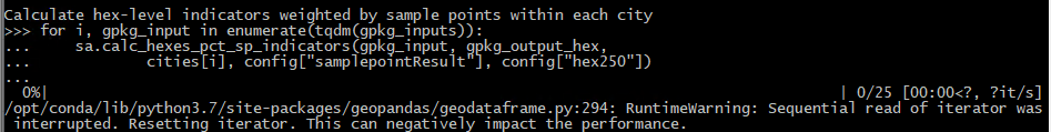
this appears to relate to an update to the fiona package which Geopandas uses when reading in data. I have found other threads discussing the issue, and that it appears to just be a performance warning not an error per se; I could not locate any fixes for addressing this:

https://stackoverflow.com/questions/64995369/geopandas-warning-on-read-file
Toblerity/Fiona#986

The warning appears multiple times when running our code, so it would be nice if it could at least be suppressed. However, i also don't think it is a priority (there is another issue with the code in aggr.py which appears to stop it running successfully, which I don't believe is related to this; so just logging this warning for reference to address later).

Opening an issue to document ideas. What can we do to make the validation most helpful for the policy team prior to hand-off?

It'd be helpful if everyone could peruse the current /validation folder and add comments here regarding:

• suggestions for additional analyses to complete
• tweaks to existing analyses
• interpretations of the how the OSM data align with the official data

for Nick and David's work this summer. I'll discuss with them and come up with a workplan.

cc @shiqin-liu @carlhiggs @duelran @nicholas-david @Dmoctezuma80

I try to extract complete OSM network: "all (non-private) OSM streets and paths", with 'graph_from_place' and 'graph_from_polygon', but it takes forever to run (for 1h+, still not responding), but it works fine for 'graph_from_address'.

Here is the code for demonstration:

places = ['Phoenix, Arizona, USA']

#retain study region boundary
def studyregion_shape(address):
    G = ox.gdf_from_places(address, buffer_dist=1e4)
    return G

#Not able to get response from either this:
W_all = ox.graph_from_place(places, network_type= 'all', retain_all = True, buffer_dist=1e4)

#Or this
studyregion = studyregion_shape(places)
polygon = studyregion['geometry'].iloc[0]
W_all = ox.graph_from_polygon(polygon, network_type= 'all', retain_all = True)

#but works fine for:
W_all = ox.graph_from_address(places, network_type= 'all', retain_all = True)

But with 'graph_from_address', we are not able to set buffer for the study region? In Carl's scripts, he suggests 10km buffer for the study region to retain all network. Not sure how that 's important, maybe we could discuss further.

I had a question regarding the validation data folders. During our meeting we discuss setting up the data on a root folder for the script to run (unzipping it first). I finished a script to unzip the data folders once the user downloads it to their own computer from the root folder. Do we need the script to be added to the main edge_validation py? Should we include all the data into different folders by city on CloudStor?

I have the following code:

import zipfile
from os import listdir, path

global_indicators_path = path.dirname(path.abspath(__file__))
edge_validation_data_path = path.join(global_indicators_path, "data", "edge_validation")
for city in listdir(edge_validation_data_path):
    with zipfile.ZipFile(path.join(edge_validation_data_path, city), "r") as zip_data:
        zip_data.extractall(path.join(edge_validation_data_path))

Looking at SpatialVision's code in sv_sp.py, I have a concern about the method they have implemented for deriving distance to amenity estimates for sample points based on association with nearby nodes.

On line 219, there is the following code:

# for each sample point, create a new field to save the osmid of the closest point,
  # which is used for joining to nodes
  samplePointsData['closest_node_id'] = np.where(
      samplePointsData.n1_distance <= samplePointsData.n2_distance,
      samplePointsData.n1, samplePointsData.n2)

  # join the two tables based on node id (join on sample points and nodes)
  samplePointsData['closest_node_id'] = samplePointsData[
      'closest_node_id'].astype(int)

  # first, join POIs results from nodes to sample points
  samplePointsData = samplePointsData.join(gdf_nodes_poi_dist,
                                           on='closest_node_id',
                                           how='left',
                                           rsuffix='_nodes1')

This appears to be saying, given the closest node, assume that because its the closest to this sample point then the distance from this node to a destination will be the best estimate for distance from this sample point to a destination. Then, it appears that the distance from the sample point to that closest node is also disregarded.

I think this is wrong in a few ways, and it would be great to get others thoughts.

Each sample point has been generated on a network edge, and as such each only has two possible nearest nodes - located at the terminating ends of the line segment.

e.g. this point is associated with nodes N1 (10 units away), and N2 (37 units away)

Line start (node 1, N1) o----------point-------------------------------------o Line end (node 2, N2)

The reason why it is invalid to just assume that the nearest node provides an adequate estimate of shortest distance to a destination is because unless access through both of these nodes is evaluated, respectively summing on the distance of the two nodes to the sample point, then the true answer of which node is closer cannot be known. SpatialVision do neither of these things; however, that is the reason they were provided with the associated nodes and the distances from the sample points, so they could calculate the two potential full minimum distances, and then take the smaller value of the two.

For example, SpatialVision's method appears to me to assign the distance from N1 to the closest supermarket directly as an estimate to the sample point. But what if the closest supermarket to both N1 and N2 is 10 units to the right of N2? That would mean the distance for N1 is 57 units, and the distance for N2 is 10 units. Taking the minimum distance from the two points alone is not sufficient --- you have to consider the distance first from the point to the nodes

Scenario A (N1): 10 + 10 +37 +10 = 67 units (including backtracking, which doesn't make sense - but its how this method works)
Scenario B (N2): 37+ 10 = 47 units

So, Scenario B shows that N2 is closer to the supermarket; you take the minimum distance of the two fully accounted for distances as the sample point's distance to closest estimate.

There is an exception to this logic --- regardless of whether N1 and N2 are closer to the supermarket, if its found that the sample point and the supermarket are both located on the same network edge, the supermarket may be closer to the sample point than either N1 or N2. It may not be the case, but it probably is and to be thorough, it could be considered.

So maybe that is
Scenario C (if sample point shares line segment with destination): Euclidean distance

Technically, a line could curve, and Euclidean distance might be wrong, but for a single edge segment we would expect any such error to be very small.

Example
Here's an applied example of how SpatialVision's method could be very problematic.

In the image below, there is a road segment 1120 metres in length, and contains 38 sample points; there are also two supermarkets nearby. The two terminal nodes are bright yellow.

The left-most node is about 380 metres from a supermarket, the right-most node is about 1100 metres away.

I think without doing the math, that to figure out which sample point on the line should go to which supermarket ... you have to do the math, adding on the full distances to the two options for each sample point, and then taking the minimum as the final answer.

In contrast SpatialVision assign half the points to node 1 ("380 metres away") and half to node 2 (1100 metres away). This actually defeats the purpose of our sampling resolution which is to have continuous estimates, but is also inaccurate: the two points in the middle of the line --- one should have been about 880 metres away (a false positive for accessibility using SV method), and the other is similar, say 910 metres (coincidentally for SV, a true negative - but they actually matched to totally different supermarkets, as the closest is accessed via N1 in both instances, despite the second node being nominally closer to N2).

What I think should be done is not much more computationally complex (as for now, I will overlook scenario C).

• replace lines 209-215 with expansion of the samplePointsData dataframe to long form, with each point having two rows (for N1, and N2), and the node IDs as recast as integers
• join with the gdf_nodes_poi_dist data frame (like on line 218)
• sum each node amenity distance to the sample point distance variable
• for each sample point, take the minimum full amenity distance of the two options

that's it! It shouldn't take much longer and would be much more accurate (it's actually my understanding of what we asked SpatialVision to do; hence why we provided them with the variables in order to calculate this, rather than just pre-associate with closest node).

There could be extension of the above to account for the occasional Scenario C situation --- that distance could perhaps be appended where applicable to the long frame result dataframe before summarising to find the minimum full distance for each amenity.

I'll see if I can implement a proof of concept version of this tomorrow - but also keen to hear your thoughts as a sanity check in case I am misreading what SpatialVision have done. I am pretty sure I'm not though...

@carlhiggs on the call today I was reminded that we still need to attach the city-level air pollution data to our indicators output. The relevant variables would be:

• E_EC2E_T15
• E_EC2O_T15
• E_EPM2_T15
• E_CPM2_T14

You have a local copy of the urban centers database, right? If so would you mind quickly attaching those columns from it to our indicators output in the code?

Hi all (esp. @shiqin-liu and @gboeing !)

I just received a security warning for the Docker requirement to use Pillow 8.0.*; apparently for versions less than 8.1.1 there's a vulnerability in the regex code that can be exploited by a malicious pdf.

I don't see it being an issue for the project per se, except that its a bad look having a dependabot warning on the repo page

I was just making those few changes to the setup_config.py for the other issue (change pre-processed study region folder from 'input' to 'study_region') --- so i just tested a rebuild of the image making the suggested requirement change
Pillow>=8.1.1

It appears to work fine for me, and I expect it will address the warning (I'm not sure what Pillow is used for exactly in the project; I expect its a dependency of one of our packages).

Are you happy for me to push this change up in both code (requirements.txt, and environment.yml) and to DockerHub?

Hi!

ISSUE: The mdillon/postgis docker image that is instructed in process/pre_process/readme.md does not seem to include pgrouting which is required in the process. Using this image results in an error at least in 00_create_database.py, and later on in 03_create_network_resources.py.

FIX SUGGESTION: I used starefossen/pgrouting instead - it is based on mdillon/postgis, but contains pgrouting readily installed. Probably not the only alternative but seems to work!

I updated the instructions in my fork, branch helsinki where I'm testing to replicate the results for Helsinki :)

The current accessibility method takes the binary approach with hard threshold, which take a rectangular function assuming the value 1 if included in a pre-defined threshold and the value 0 if not (refer here to the code). This method is appropriate for our purpose of indicator aggregation using open data, and passes the suitability analysis in the validation.

But there is also limitation to this approach, since it assumes that if a destination is slightly farther away from the origin (even by only 2 m: 499m vs 501m) it will have a lower attraction. Thus, there could be improvement in our accessibility measures to allow for custom linear distance decay function. From the literature, I found two methods may be applicable to our framework:

1. Cumulative–Gaussian function: which combines the rectangular function to model the acceptable distance threshold up to a value of perceived closeness, then apply a modified Gaussian function that reflects the influence of distance beyond that acceptable threshold.

Reference: Vale, D. S., & Pereira, M. (2017). The influence of the impedance function on gravity-based pedestrian accessibility measures: A comparative analysis. Environment and Planning B: Urban Analytics and City Science, 44(4), 740–763. https://doi.org/https://doi.org/10.1177/0265813516641685

2. Soft threshold approach: which defines a continuous access score for each destination type ranging from 0 to 1

Higgs, C., Badland, H., Simons, K. et al. The Urban Liveability Index: developing a policy-relevant urban liveability composite measure and evaluating associations with transport mode choice. Int J Health Geogr 18, 14 (2019). https://doi.org/10.1186/s12942-019-0178-8)

We discussed the second option before on basecamp, @carlhiggs you may have more thoughts on this since you are the authors of the approach.

I haven't implement these within our framework yet, but want to share the thought process so far, and keen to hear others suggestion on this.

Hello, I'm interesting in this project.
In the past few days, I have tried to make the code run successfully on my machine.
Now I'm wondering if it is convenient to get the dataset?
No matter what the answer is, I appreciate all of your work.
Thanks

@shiqin-liu there appears to be a bug in /process/sp.py on this line, but I want to confirm with you.

Specifically, it saves the "samplepointResult" results layer to gpkgPath rather than gpkgPath_output. This means that the results are being saved to the input file, such as olomouc_cz_2019_1600m_buffer.gpkg but it appears that they should be getting saved to the output file instead, such as olomouc_cz_2019_1600m_buffer_output20200402.gpkg, right?

For example, running aggr.py throws an exception, because it cannot find the "samplepointResult" layer in olomouc_cz_2019_1600m_buffer_output20200402.gpkg.

David and I have been looking through the data on Cloudstor, and we are unable to find the official data for Olomouc's edges. For Olomouc's official data, we were only able to find supermarket destination data. Is anyone able to send the original official data for Olomouc?

@gboeing @carlhiggs

I'm trying to run the notebooks but seem to be unable to access the CloudStor data without a password?

Dependabot alerts have been generated for pillow and jupyterlab versions currently used in our Docker image.

https://github.com/global-healthy-liveable-cities/global-indicators/security/dependabot/docker/requirements.txt/pillow/open
https://github.com/global-healthy-liveable-cities/global-indicators/security/dependabot/docker/requirements.txt/jupyterlab/open

To resolve, it is recommended to use
pillow>=8.3.2
jupyterlab>=2.2.10

Currently
pillow == 8.2.*
jupyterlab == 2.1.*

Before updating to fixed versions in the above recommended ranges, it should be confirmed that our code remains stable

Need to confirm that city-linkage with Global Human Settlements Urban Centres database air pollution covariates is correct. A question was raised that this may be matching on city name, but not country name, resulting in inaccuracies for two cities for those statistics, including marginal estimates --- this needs to be confirmed, and resolved if there are issues to ensure statistics are accurate.

Hi!

Running _create_preliminary_validation_report.py in the default environment results in ExtensionError: You must configure the bibtex_bibfiles setting.

Seems that the latest version of sphinxcontrib-bibtex is incompatible with some other stuff.

I now manually downgraded to sphinxcontrib-bibtex==1.0.0 and managed to build the PDF, but apparently a better fix would be to restrict the package vesrion in requirements.txt like this: sphinxcontrib-bibtex<2.0.0 as discussed in here: executablebooks/jupyter-book#1137.

Cheers :)

It appears that sample points are being used for weighting of population percent access measures, rather than population (at least in the language of the functions). It will be good to verify that we are usuing population estimates, not sample point counts, to weight our indicators. While these may be correlated in some instances, sample point counts are a direct function of road length (generated at regular intervals along network, except where located within identified public open spaces); as such, they are not our best estimate for location of population.

e.g. in setup_aggr.py

def calc_hexes_pct_sp_indicators(gpkg_input, gpkg_output, city, layer_samplepoint, layer_hex): """ Caculate sample point weighted hexagon-level indicators within each city, and save to output geopackage

-- we need to make sure that both the data used and the language representing the data are in terms of population, not sample points (ie. not our units of interest).

@gboeing @carlhiggs

I am running the aggregation script for 10 cities. The code is not completing though, this is what I am getting

Process aggregation for hex-level indicators.

Cities: ['adelaide', 'baltimore', 'bern', 'ghent', 'lisbon', 'mexico_city', 'odense', 'olomouc', 'valencia', 'vic']

Calculate hex-level indicators weighted by sample points within each city
0%| | 0/10 [00:00<?, ?it/s- 'VirtualXPath' [XML Path Language - XPath]
0%| | 0/10 [00:00<?, ?it/s]
Traceback (most recent call last):
File "aggr.py", line 60, in
cities[i], config["samplepointResult"], config["hex250"])
File "/home/jovyan/work/process/setup_aggr.py", line 37, in calc_hexes_pct_sp_indicators
gdf_samplepoint = gpd.read_file(gpkg_input, layer=layer_samplepoint)
File "/opt/conda/lib/python3.7/site-packages/geopandas/io/file.py", line 96, in _read_file
with reader(path_or_bytes, **kwargs) as features:
File "/opt/conda/lib/python3.7/site-packages/fiona/env.py", line 400, in wrapper
return f(*args, **kwargs)
File "/opt/conda/lib/python3.7/site-packages/fiona/init.py", line 257, in open
layer=layer, enabled_drivers=enabled_drivers, **kwargs)
File "/opt/conda/lib/python3.7/site-packages/fiona/collection.py", line 164, in init
self.session.start(self, **kwargs)
File "fiona/ogrext.pyx", line 549, in fiona.ogrext.Session.start
ValueError: Null layer: 'samplePointsData'

Do you know why this is happening? I downloaded the GTFS data and the input data from the cloudstor, so I am not sure what is happening. Thanks for the help

@gboeing @carlhiggs

For the process data, the data organization on cloudstor is a little confusing. I think it would be positive if all the data could be downloaded in one click. That would involve moving the old input data out of the input folder, and incorporating the most recent GTFS data into the input folder. Please let me know your thoughts. I will make sure to update the documentation according to what you implement.

When running the docker batch script which included a git pull command, the warning came up

Your configuration specifies to merge with the ref 'refs/heads/full_dist_function' from the remote, but no such ref was fetched.

I expect this probably isn't an issue that will impact things, but in case it hadn't been noted, sharing here (not sure how to address this myself).

The current set of project requirements are quite complex, partly because the software

• tries to do many things (e.g. different analyses and reporting on these in different formats)
• had multiple authors working on different components (tasks could be more refactored with dependencies streamlined)
• developed out of previous projects, with their own histories of the above

I think it could be good to consider seperating out the analysis (focus on that in this repository) and reporting in multiple formats (that could be the task of the global-scorecards repository), at least while things are re-factored.

I've created a tagged version of the software as it was for our preliminary 25 city analysis, but now we are planning to use the tools more broadly, I think it would be good to think about how to refine these aspects.

When i was thinking about this earlier in the year, I made the following diagram which illustrates how reporting can be considered a bit of a seperate concern from the analysis which generates the underlying data. Perhaps if we seperate these things (the database, the analysis, and the reporting), it'll make it easier to re-factor / simplify how each of these aspects are seperately conducted. Then later, we might be able to re-integrate them in a single software package.

Regarding the database, currently we use a mix of data storage formats (including PostgreSQL+PostGIS and geopackage); this is also something we could simplify and streamline (eg only output the final outputs to geopackage, but otherwise work connecting directly to the SQL database, may be more efficient with faster read/write and fewer artifacts).

This isn't something to rush into, but I'm posting this here as something to think about and discuss; what do you think @gboeing @shiqin-liu @duelran @VuokkoH ?

When re-running the aggregation code after re-processing Bangkok (to add in analysis of a recently located GTFS feed for that city, to help with global comparisons), a bug was encountered which causes the analysis not to sucessfully run.

Specifically, I have found that the incompatibility is a key look up error where a subset of relevant fields are requested to be retained after reading in the sample point geopackage layer for a city.

The error looks like this, when processed interactively from within the calc_hexes_pct_sp_indicators() function:

The fields that are requested are:

>>> ['hex_id']+sc.fieldNames_from_samplePoint
['hex_id', 'sp_access_fresh_food_market_score', 'sp_access_convenience_score', 'sp_access_pt_osm_any_score', 'sp_access_public_open_space_any_score', 'sp_access_public_open_space_large_score', 'sp_access_pt_gtfs_any_score', 'sp_access_pt_gtfs_freq_30_score', 'sp_access_pt_gtfs_freq_20_score', 'sp_access_pt_any_score', 'sp_local_nh_avg_pop_density', 'sp_local_nh_avg_intersection_density', 'sp_daily_living_score', 'sp_walkability_index']

And the fields present in the layer which don't match these are:

>>> [x for x in gdf_samplepoint.columns if x not in ['hex_id']+sc.fieldNames_from_samplePoint]
['point_id', 'edge_ogc_fid', 'sp_nearest_node_fresh_food_market', 'sp_nearest_node_convenience', 'sp_nearest_node_pt_osm_any', 'sp_nearest_node_public_open_space_any', 'sp_nearest_node_public_open_space_large', 'sp_nearest_node_pt_gtfs_any', 'sp_nearest_node_pt_gtfs_freq_30', 'sp_nearest_node_pt_gtfs_freq_20', 'sp_access_fresh_food_market_binary', 'sp_access_convenience_binary', 'sp_access_pt_osm_any_binary', 'sp_access_public_open_space_any_binary', 'sp_access_public_open_space_large_binary', 'sp_access_pt_gtfs_any_binary', 'sp_access_pt_gtfs_freq_30_binary', 'sp_access_pt_gtfs_freq_20_binary', 'sp_access_pt_any_binary', 'geometry']

The mismatch apparently relates to the anticipation of variables with suffix 'score', where the recorded variables have suffix 'binary'.

The suffix for these variables (listed in the variable fieldNames_from_samplePoint) was changed in the setup_config.py code in February 2021 here.

However, with the exception of Bangkok and Sydney which I have re-processed (based on updated GTFS results) the other cities were processed in October, meaning their sample point output layers contain variables with the suffix 'binary' and so there is a failure when variables with suffix 'score' is anticipated.

So ---- having thought through the above while writing, the fix seems pretty obvious: re-run the sample point analyses for all cities. That actually shouldn't take too long, I believe as the node relations don't need to be re-processed; from memory the re-processing of Sydney the other day only took 16 minutes or so. So, I'll do that and update here to confirm that the re-processing of results according to the updated name schema has successfully resolved this issue.

It has been noted that all_cities_walkability at city level is still based on sum of marginal z-scores (street density, intersection density, daily living score), rather than two seperate measures for average and population weighted average of the hex-level sums of z-scores.

As per this post
https://3.basecamp.com/3662734/buckets/11779922/messages/2465025799
it was agreed we would calculate both spatial and population based measures of walkability

As I mentioned in PR #49, there is a warning message when running the current workflow:

/opt/conda/lib/python3.7/site-packages/pyproj/crs/crs.py:53: FutureWarning: '+init=<authority>:<code>' syntax is deprecated. '<authority>:<code>' is the preferred initialization method. When making the change, be mindful of axis order changes: https://pyproj4.github.io/pyproj/stable/gotchas.html#axis-order-changes-in-proj-6
  return _prepare_from_string(" ".join(pjargs))

In future work, we should use for example "to_crs": "epsg:7845" but not "to_crs": { "init": "epsg:7845" } to define projection, as the warning suggests. I updated all the CRS format in the current GitHub workflow, but the warning message is still there. So there should be some old-style "init" in the data.

@carlhiggs I have checked the upstream repository for the input data source, 'init' format is used when creating the population grid (in 06_create_population_grid.py). Since the warning still exists, this issue is created to remind us that we should update the CRS syntax throughout the workflow when reproducing the data.

Currently, the intersection cleaning/consolidation process uses a single tolerance parameter across the entire project, with a default of 12 metres. This is used to ensure that representation of features such as roundabouts don't bias estimates for street connectivity upwards due to excessive node artifacts; instead, the network is simplified by some tolerance value.

The current default of 12m was used following review of networks in different contexts (e.g. dense inner city laneways, and sprawling outer suburban neighbourhoods with cul-de-sacs) in the Australian context, and appeared to perform adequately in our preliminary 25-city study.

However, when this was applied to Helsinki (by @VuokkoH, see https://github.com/VuokkoH/osmnx-intersection-tuning/blob/main/osmnx-intersection-tuning-helsinki.ipynb ), it was found that a 5m tolerance was more appropriate due to the dense and detailed way that OpenStreetMap had been used to represent urban features in that context.

This means that we should consider allowing some city-specific tuning of the tolerance parameter, to ensure the representation of cleaned intersections best represents the reality on the ground. The risk is that street connectivity would be evaluated in a different way in different cities, causing problems for comparability. However, as Vuokko's investigations demonstrate, in the Helsinki context the 12m tolerance leads to visibly apparent over-cleaning and hence under-estimation of true connectivity. As such, allowing city-specific tuning appears the most sensible option.

This will involve modifying the pre-process script _project_setup.py to read a city-specific parameter defined in region_settings instead of project_settings of the project configuration file _project_configuration.xls.

This should be straightforward to implement; i'll aim to do this in the coming week.

When we execute 01_create_study_region.py, the defined boundaries 'boundaries.gpkg' is not found. Please see the following error notice:

Traceback (most recent call last):
Create study region boundary...
Traceback (most recent call last):
File "fiona/_shim.pyx", line 83, in fiona._shim.gdal_open_vector
File "fiona/_err.pyx", line 291, in fiona._err.exc_wrap_pointer
fiona._err.CPLE_OpenFailedError: .././data/boundaries.gpkg: No such file or directory

Hi all,
I have completed my cities, however, there are some issues I found with Phoenix, Chanai and olomouc after aggregating the result. I only get partial hex grid results as shown below for example:

Phoenix:

So I checked the dataset,  somehow the samplePointsData_droped_nan layer is much larger than the samplePointsData layer. That means it is possible that the process dropped sample point data that should not be dropped in the dataset. In sv_sp.py: 

samplePointsData_withoutNan = samplePointsData.dropna().copy() 

When checking samplePointsData_droped_nan layer, I found the column ref empty (see below) while all else is complete. So my best guess is that the process dropped all those NA data because of this. The ref column seems to come from the nodes layer in the input dataset.

I am not sure why this only happens to some cities but not others. (with other normal ones, the ref column is often filled with Nan values rather than showing as empty like this). If this is the real problem, I guess it should be relatively easy to fix. I have run phoenix and Olomouc twice to make sure it is not just an incident. I also run the file that Geoff has uploaded on the cloud drive. And I found similar problems too,

for example, Melbourne:

Can anyone check the output layer and confirm if this problem also occurs to you?

When looking to analyse the recently located GTFS feed for Bangkok, we found that despite the feed appearing to be complete and full of data, when subjected to the restrictions of our analysis workflow too few stops were identified.

On investigation, it was found that the get_hlc_stop_frequency() function's filtering of the frequencies.txt data (which for Bangkok defines headways for specific trips) failed to match integer trip IDs to string-formatted trip IDs for the mode-specific routes of interest. This resulted in most stops being wrongly excluded, where if the match was understaken forcing both ID variables to be strings, the analysis succeeds as intended.

I am posting this issue as a record of this, prior to pushing up a fix to address it.

Should we save the OSM output for Pheonix at this point? For now, I try to save the network output just for experimental purpose. Two quick questions:

1. Should I save graphs as shapefile or GraphML? Not so familiar with GraphML...

2. How can I save in a folder a level up a directory? For example, I am currently under the process folder, how can I save the output in a new folder under the parent directory global-indicator if using ox.save_graph_shapefile?

Let me know if saving the output is not necessary at this point.

Thank you!