hadley / r4ds Goto Github PK
View Code? Open in Web Editor NEWR for data science: a book
Home Page: http://r4ds.hadley.nz
License: Other
R for data science: a book
Home Page: http://r4ds.hadley.nz
License: Other


When I run the command in the introduction page to install the required packages, I get the following warning:
Warning in install.packages :
  package 'modelr' is not available (for R version 3.3.1)
I checked the CRAN repo - and did not find modelr there either.
I found the modelr github page, and followed the instructions there to install from github directly.
16.1.1 Exercises, exercise 2
Hi Hadley,
Huge thanks for putting this book out there, amazing work as always. I've been going through the regex section (11.4.5) , and noticed what I believe is an error below
x <- c("1 house", "2 cars", "3 people")
str_replace_all(x, c("1" = "one", "2" = "two", "3" = "three"))
#> [1] "one house"  "one cars"   "one people"
Judging from the context, I think you want str_replace_all in this case to produce
#> [1] "one house" "two cars" "three people"
But it seems to be instead applying the first replacement to all matches? Suppose this is a stringr issue but thought it would be easier to point out here.
In 4.3 Filter rows with filter(),
filter() works similarly to subset() except that you can give it any number of filtering conditions, which are joined together with &.
Does it actually mean "you can give it any number of filtering conditions separately, which are joined together with & automatically behind scene"? Because if you are giving one huge expressions with multiple conditions joined, it should work with both filter() and subset().
In 4.3.2 Logical operators
Multiple arguments to filter() are combined with “and”.
Should it be this?
Multiple arguments to filter() are combined with “&”.
I started writing you an email about this but felt it was better suited for here. I hope that was the correct decision.
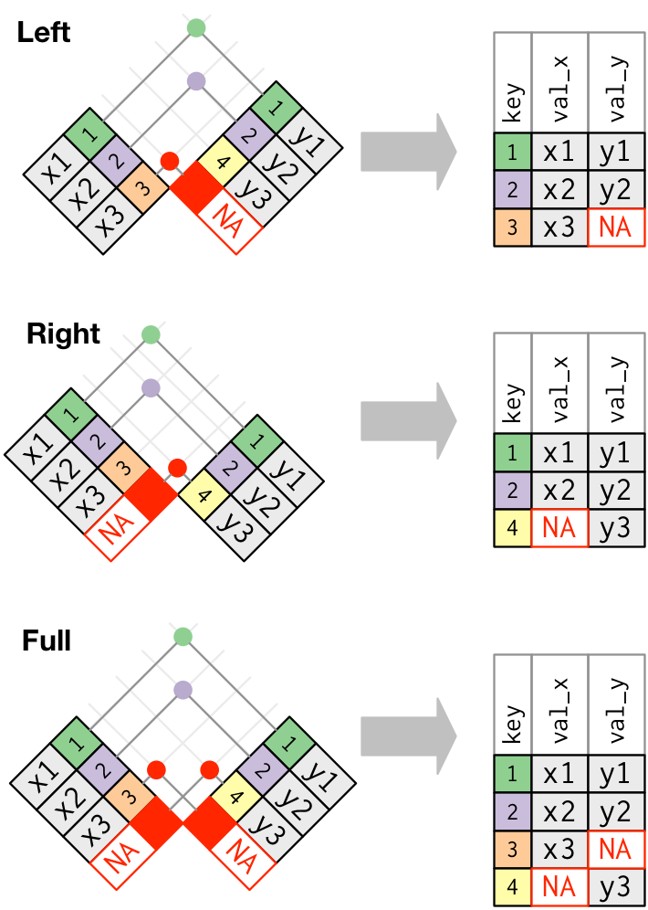
The join diagrams you have so far are really great. You've thought about this a lot more than me, so I'll throw out some ideas and a few questions:
Question 1
Is there a difference between an inner_join(x, y) and semi_join(x, y)?
The only thing I can see is that the columns that are not joined by in y are dropped:
Using your DS4R example:
require(dplyr); require(nycflights13)

top_dest <- flights %>% # getting top ten destinations
    count(dest, sort = TRUE) %>%
    head(10)

semijoined <-flights %>% semi_join(top_dest)
flights %>% inner_join(top_dest)

flights %>% inner_join(top_dest) %>% anti_join(semijoined) #no different rows 0x17
flights %>% inner_join(top_dest) %>% anti_join(semijoined, .) #no different rows 0x16
#dropped n column from top_dest
Opinion 1
Representation of semi_join() should be the same as an inner_join().

In this example, there are literally no difference between the two.
x <- data_frame(key = c(1, 2, 3), val_x = c("x1", "x2", "x3"))
y <- data_frame(key = c(1, 2, 4), val_y = c("y1", "y2", "y3"))
semi_join(x, y, by="key")
I'd love to know if I'm missing something.
Opinion 2
Representation of the anti_join() could use the full join figure.
http://r4ds.had.co.nz/diagrams/join-outer.png

In the case of anti_join(x,y) you would only get the 3-X3 row as the output. I don't think it needs to be more complex than that.
Question 2
Is there such a thing as a full_anti_join?
In this case, you would get rows that exist in x and aren't in y and rows that aren't in x but exist in y. Essentially:
full_join(anti_join(x,y), anti_join(y,x))Comment 1
In the join.graffle file, I had to uncheck "wrap to shape" to get the NAs to fit in their boxes. Not sure why it looks great on the site and messed up in the file.
Note: I got this error when trying to "Build the Book." I was able to finally compile the book after installing and loading the broom package and the curl package.
Thank you for a great book!
In the chapter functions.Rmd, you write
This fails because it tells dplyr to group by group_var and compute the mean of mean_var neither of which exist in the data frame. Writing reusable functions for ggplot2 poses a similar problem because aes(group_var, mean_var) would look for variables called group_var and mean_var. It's really only been in the last couple of months that I fully understood this problem, so there aren't currently any great (or general) solutions.
So I'm just wondering if there is any solution to write that kind of functions. I think it would be really valuable for everyone.
xor (x,y) is unclear and not consistent with the other logical transformations. Should it be !(x & y)?
The transform chapter in the online version (http://r4ds.had.co.nz/transform.html) currently has some wrong figures from the plotting chapter.
In Chapter 11 Dates and times, under the section "11.1.0.1 The structure of dates and times", near the end of this section:
"This gives us a way to calculate the scheduled departure and arrival times of each flight in flights." together with the following code block.
I think this part is in fact calculating the actual departure and arrival times, not the scheduled times, of the nyc flights data.
Just thought I should highlight this. Thank you.
Hi Jenny,
i'm using googlehsheets in R. .there is some issues when I tried to use .rds for authentication without interaction with browser. it seems failed refreshing and I have to use gs_auth() to re-enter my authentication in browser.
gs_auth(token = "ttt.rds", verbose = FALSE)
Auto-refreshing stale OAuth token.
Error in function_list[k] : Unauthorized (HTTP 401).
In addition: Warning message:
Unable to refresh token
I have been trying trying to use bookdown to render the files into a single pdf from a console session without using RStudio.
Is it possible to get some steps to do this added?
In section 16.2.4 Unknown sequence length, this example code:
flip <- function() sample(c("T", "H"), 1)

flips <- 1
nheads <- 0

while (nheads < 3) {
  if (flip() == "H") {
    nheads <- nheads + 1
  } else {
    nheads <- 0
  }
  flips <- flips + 1
}
flips
I think setting nheads <- 0 in the else construct is not correct.
Also shouldn't we start with flips <- 0 ?
This question is acutally about RStudio, not really about the book, but I wanted to post here because posts in RStudio support often have no response for long time.
I found the syntax highlighting theme for code in book very informative. Once the code in book was copied to RStudio, they become rather dull with same color for almost everything. Two very helpful differences are the known library function names (bold green) and the function parameter assignments (dark red).
The theme in book seemed to be implemented by customized CSS, but there should be no difficulty to implement similar effect in RStudio. I searched RStudio support and found several similar requests dated as early as 2013.
I submitted a feature request in RStudio support
I love "shiny" for rapid prototypeing. However, in production based context the OpenCPU API (http://www.opencpu.org) is a valuable alternative, that does not only scale well but also enables to separate backend (R package) from front-end development. Thus I really appreciate if you spread a word about the OpenCPU alternative in your upcoming book.
Rmarkdown and shiny chapters will talk about communicating with other humans, but it's probably worthwhile to think about what a chapter about communicating with other programs might look like. By parallel to the import section, it might contain:
(To be comprehensive, it would probably need a decent amount of software engineering, since, e.g., readxl currently doesn't do exports)
In 4.8 Grouped mutates (and filters), if the worst member means the flight with most delays,
# Find the worst members of each group:
flights %>%
  group_by(year, month, day) %>%
  filter(rank(arr_delay) < 10)
This seemed to be the flights that with least delays, i.e. negative arr_delay, but the code example doesn't show arr_delay column so it is not obvious.
> flights %>%
+   group_by(year, month, day) %>%
+   filter(rank(arr_delay) < 10)
Source: local data frame [3,360 x 19]
Groups: year, month, day [365]

    year month   day dep_time sched_dep_time dep_delay arr_time sched_arr_time arr_delay carrier flight tailnum origin
   (int) (int) (int)    (int)          (int)     (dbl)    (int)          (int)     (dbl)   (chr)  (int)   (chr)  (chr)
1   2013     1     1      820            820         0     1249           1329       -40      DL    301  N900PC    JFK
2   2013     1     1      840            845        -5     1311           1350       -39      AA   1357  N5FSAA    JFK
3   2013     1     1     1153           1200        -7     1450           1529       -39      DL    863  N712TW    JFK
4   2013     1     1     1245           1249        -4     1722           1800       -38      DL    315  N670DN    JFK
So the flights with most delays should be
> flights %>%
+   group_by(year, month, day) %>%
+   filter(rank(-arr_delay) < 10)
Source: local data frame [3,306 x 19]
Groups: year, month, day [365]

    year month   day dep_time sched_dep_time dep_delay arr_time sched_arr_time arr_delay carrier flight tailnum origin
   (int) (int) (int)    (int)          (int)     (dbl)    (int)          (int)     (dbl)   (chr)  (int)   (chr)  (chr)
1   2013     1     1      848           1835       853     1001           1950       851      MQ   3944  N942MQ    JFK
2   2013     1     1     1815           1325       290     2120           1542       338      EV   4417  N17185    EWR
3   2013     1     1     1842           1422       260     1958           1535       263      EV   4633  N18120    EWR
4   2013     1     1     1942           1705       157     2124           1830       174      MQ   4410  N835MQ    JFK
i.e. how to get it and how to read it
line 159 in visualize.Rmd
To set an aesthetic manually, do not plce it in the aes() function.
should be place
Hi there, I was reading the section on tidy data just now and I think it's a great workup of both concept and package.
The only thing that I think you might want to change is the sentence
An implicit missing value is the presence of an absence; an explicit missing value is the absence of a presence.
where explicit and implicit should trade places.
As a reference, I think the book for ggplot2 got it right where it says:
An
NAis the presence of an absence; but sometimes a missing value is the absence of a presence.
Finally, a big thanks for writing this book, it's got a great deal of refreshing clarity.
Best,
David Wolski
Hi, I have difficulty understanding the last bullet in 4.1. There's an argument that unlike a data.frame, an object of type tbl_df does not do partial matching. But the output shows it actually does partial matching. I had expected, that:
df <- data.frame(abc = 1)
df$a
would have resulted in 1.
And that
df2 <- data_frame(abc = 1)
class(df2)
df2$a
would resulted in NULL.
Actually both, result in: 1
Thanks, Richard
In 4.7.2 Missing values, not cancelled flights are defined as
not_cancelled <- filter(flights, !is.na(dep_delay), !is.na(arr_delay))
However there are some mismatches of the NAs in time and delay:
| dep_time NA's | dep_delay NA's | arr_time NA's | arr_delay NA's |
|---|---|---|---|
| 8255 | 8255 | 8713 | 9430 |
The much bigger number of arr_delay NA's turned out to be errors that can be recovered:
> flights %>%
+   filter(!is.na(arr_time), is.na(arr_delay)) %>%
+   select(dep_time:flight)
Source: local data frame [717 x 8]

   dep_time sched_dep_time dep_delay arr_time sched_arr_time arr_delay carrier flight
      (int)          (int)     (dbl)    (int)          (int)     (dbl)   (chr)  (int)
1      1525           1530        -5     1934           1805        NA      MQ   4525
2      1528           1459        29     2002           1647        NA      EV   3806
So we can just recalculate arr_delay for these records. After the recalculation, a better definition of not cancelled flights could be:
not_cancelled <- filter(flights, !is.na(dep_time), !is.na(arr_time))
Of course this may be more suit for a different topic or chapter.
Prompt. Output marker + value.
Continuation
Somewhere around here might be a good place to suggest building a plot line by line, and viewing the output of each stage to fix any problems before moving on.
I'd consider mentioning the automatic syntax checking in RStudio and that readers should make sure to eliminate any red Xs. Some might not know that hovering over a red X provides an explanation.
Cmd + return sends current statement (in preview) to the console
On the matching of () and {}, it might be good to mention that in RStudio if you put the cursor after a (, ), {, or } that the matching punctuation will be highlighted.
Tab completion
It’s good for students to know about Session > Set Working Directory. Sometimes they will open up a file in one directory and then another file in another directory, but can't understand why their code isn’t finding the files it is trying to read.
Use projects for bigger stuff
In exercise 3 of 16.2.5 Exercises, the code didn't update mtcars[["am"]] as expected in my configuration. I changed the column updating code to print, thus we can test the function without lost of original information.
data("mtcars")
trans <- list(
  disp = function(x) x * 0.0163871,
  am = function(x) {
    factor(x, levels = c("auto", "manual"))
  }
)
for (var in names(trans)) {
  print(trans[[var]](mtcars[[var]]))
}
#>  [1] 2.621936 2.621936 1.769807 4.227872 5.899356 3.687098 5.899356 2.403988 2.307304 2.746478
[11] 2.746478 4.519562 4.519562 4.519562 7.734711 7.538066 7.210324 1.289665 1.240503 1.165123
[21] 1.968091 5.211098 4.981678 5.735485 6.554840 1.294581 1.971368 1.558413 5.751872 2.376130
[31] 4.932517 1.982839
 [1] <NA> <NA> <NA> <NA> <NA> <NA> <NA> <NA> <NA> <NA> <NA> <NA> <NA> <NA> <NA> <NA> <NA> <NA>
[19] <NA> <NA> <NA> <NA> <NA> <NA> <NA> <NA> <NA> <NA> <NA> <NA> <NA> <NA>
Levels: auto manual
Calling factor directly seemed to be working:
var = "am"
factor(mtcars[[var]], labels = c("auto","manual"))
#> [1] manual manual manual auto   auto   auto   auto   auto   auto   auto   auto   auto
[13] auto   auto   auto   auto   auto   manual manual manual auto   auto   auto   auto
[25] auto   manual manual manual manual manual manual manual
But calling the function from the list didn't work:
trans[["am"]]
#> function(x) {
    factor(x, levels = c("auto", "manual"))
  }
mtcars[["am"]]
#> [1] 1 1 1 0 0 0 0 0 0 0 0 0 0 0 0 0 0 1 1 1 0 0 0 0 0 1 1 1 1 1 1 1
trans[["am"]](mtcars[["am"]])
#> [1] <NA> <NA> <NA> <NA> <NA> <NA> <NA> <NA> <NA> <NA> <NA> <NA> <NA> <NA> <NA> <NA> <NA> <NA>
[19] <NA> <NA> <NA> <NA> <NA> <NA> <NA> <NA> <NA> <NA> <NA> <NA> <NA> <NA>
Levels: auto manual
In 5.2.1 Visualizing distributions
If you wish to overlay multiple histograms in the same plot, I recommend using geom_freqpoly() or geom_density2d()
geom_density2d() should be geom_density()
I like dplyr and tidyr. Those packages are really useful to work with conventional tabular data sets. However, we should add recommandations to work with specific data sets such as geographical data (polygons of cities, countries, etc) or network data.
For geographical data, SpatialPolygonsDataFrame aren't easy to manipulate. For instance, it's not very handy to filter a SpatialPolygonDataFrame. Converting SpatialPolygonDataFrame to data frames (what we do with fortify to draw polygons using ggplot2) isn't the best solution for memory usage. SO we might be able to find something else and have good recommandations for data-scientists.
I recently had to work with network data. It was also very difficult to find the good structure for my data. Imagine I have a dataset with in the first column the set of each node and in the second column a list of groups the node belongs to. I want to have a data set with one line for each relationship between two nodes (I assume that if node A and node B belong to group 1, they have 1 relation). Standard tools such as tidyr are not really done for that kind of usage.
I think that those kind of data are very often used by data-scientists and this book should also address those issues.
In the Data Transformation chapter, the following is written:
$, tbl_dfs never do partialdf <- data.frame(abc = 1)
df$a
df2 <- data_frame(abc = 1)
df2$aHowever the live version of the r4ds website (immediately above http://r4ds.had.co.nz/transform.html#dplyr-verbs) implies that partial matching does work. At any rate, it doesn't throw an error, as was meant to be illustrated.
I get the same in my R console:
df <- data.frame(abc = 1)
df$a
#> [1] 1

df2 <- data_frame(abc = 1)
df2$a
#> [1] 1
Do tbl_dfs now do partial matching with $?
FYI:
sessionInfo()
#> R version 3.2.4 (2016-03-10)
#> Platform: x86_64-apple-darwin13.4.0 (64-bit)
#> Running under: OS X 10.11.4 (El Capitan)
#>
#> locale:
#> [1] en_US.UTF-8/en_US.UTF-8/en_US.UTF-8/C/en_US.UTF-8/en_US.UTF-8
#>
#> attached base packages:
#> [1] stats     graphics  grDevices utils     datasets  methods   base
#>
#> other attached packages:
#> [1] reprex_0.0.0.9001 dplyr_0.4.3
#>
#> loaded via a namespace (and not attached):
#>  [1] Rcpp_0.12.4     knitr_1.12.3    magrittr_1.5    splines_3.2.4
#>  [5] MASS_7.3-45     lattice_0.20-33 R6_2.1.2        minqa_1.2.4
#>  [9] stringr_1.0.0   tools_3.2.4     parallel_3.2.4  grid_3.2.4
#> [13] nlme_3.1-125    DBI_0.3.1       clipr_0.2.0     htmltools_0.3.5
#> [17] lme4_1.1-11     lazyeval_0.1.10 assertthat_0.1  digest_0.6.9
#> [21] Matrix_1.2-4    nloptr_1.0.4    formatR_1.3     evaluate_0.8.3
#> [25] rmarkdown_0.9.5 stringi_1.0-1In chapter 5.4 I would suggest to use "if_else" from the dplyr package instead of "ifelse".
Uptil that point, ggplot call passed the mapping to the geom_point call. For example:
ggplot(data = mpg) +
  geom_point(mapping = aes(x = displ, y = hwy))
In the first example of 3.5, though, the mapping is specified on the ggplot call instead:
ggplot(data = mpg, mapping = aes(x = displ, y = hwy)) +
  geom_point() +
  facet_wrap(~ class, nrow = 2)
It may be useful to clarify what the difference between the two approaches might be.

In the above screenshot flights2 <- flights %>% select(year:day, hour, origin, dest, tailnum, carrier) and flights2 %>% left_join(airlines, by = "carrier") output the same table, if I run the code for the second line in my computer I get the correct output:
Source: local data frame [336,776 x 9]

    year month   day  hour origin  dest tailnum carrier                     name
   (int) (int) (int) (dbl)  (chr) (chr)   (chr)   (chr)                   (fctr)
1   2013     1     1     5    EWR   IAH  N14228      UA    United Air Lines Inc.
2   2013     1     1     5    LGA   IAH  N24211      UA    United Air Lines Inc.
3   2013     1     1     5    JFK   MIA  N619AA      AA   American Airlines Inc.
4   2013     1     1     5    JFK   BQN  N804JB      B6          JetBlue Airways
5   2013     1     1     5    LGA   ATL  N668DN      DL     Delta Air Lines Inc.
6   2013     1     1     5    EWR   ORD  N39463      UA    United Air Lines Inc.
7   2013     1     1     5    EWR   FLL  N516JB      B6          JetBlue Airways
8   2013     1     1     5    LGA   IAD  N829AS      EV ExpressJet Airlines Inc.
9   2013     1     1     5    JFK   MCO  N593JB      B6          JetBlue Airways
10  2013     1     1     5    LGA   ORD  N3ALAA      AA   American Airlines Inc.
..   ...   ...   ...   ...    ...   ...     ...     ...                      ...
I could not figure out what's wrong in the script so I leave it to the experts.
To store any datasets, and to make it easier for people to get all the packages they need.
Bottom right code snippet should be a[[4]][[1]] instead of a[[4]][1] in diagrams/lists-subsetting.png
https://github.com/hadley/r4ds/blob/56176ea369ecc03bc35d516a2003aee45eb2c467/model-basics.Rmd
In the exercise below, it's not clear to me what being compared (when you're asking about the advantages and disadvantages). Are you asking about absolute vs relative residuals? Are you asking about a frequency polygon vs some other geom/approach?
Why might you want to look at a frequency polygon of absolute residuals? What are the advantages? What are the disadvantages?
Explore the distribution of price. Do you discover anything unusual or surprising? (Hint: Carefully think about the binwidth and make sure you.)
The Hint is incomplete
From ggplot(data) + geom_...(mapping) to ggplot(data, mapping)
Some feedback as requested on Hadley's Twitter:
I think the chapter is well written, but lacks one thing: what if the function cannot do its work?
An example is a function to calculate a variance:
calculate_variance <- function(x) {
  if (length(x) < 2) {
    stop("calculate_variance: cannot calculate the variance if x has less than two values")
  }
}
Note how I add my personal preference for also adding the function its name to the error message. An alternative would be to return NA. But references [1,2] argue you should use stop.
It would be great to see some more guidance on how to handle incorrect function arguments!
Good luck, Richel Bilderbeek
Hi,
In the Function part of the book line 218:
This is an important part of the “do no repeat yourself” (or DRY) principle. The more repitition you have in your code, the more places you need to remember to update when things change (and they always code!), and the more likely you are to create bugs over time.
I am not sure if and they always code! means and they always do! . It as I understand it.
If not, this sentence is not so clear.
Sorry I could not improve myself, I am not sure of the meaning.
Thanks.
And have an index somewhere
The code in 21.1 need library tidyr because of expand(), but tidyr is not included in Prerequisites. Actually ggplot2 is also needed but not included, though that is kind of obvious.
Is it possible to have some shortcut to load libraries in Hadleyverse? For example, a line like load("wrangle") will load tidyr, dplyr, stringr,lubridate etc, load("model") will load all previous libraries plus modelr, ggplot2, and load("Hverse") load all current Hadleyverse packages.
I'm also using pacman because it can install packages if not already installed, so it's possible to run same code in other machine(all the library() lines will not run if not available already). It's not perfect yet but I didn't find better solution.
Hi,
I don't know if this is intentional or not, but the there is an exercise to detail the differences between if and ifelse, but you haven't discussed ifelse explicitly in this chapter (apologies if this is in an earlier chapter).
Load immediately after introduction? Should be visible to reader.
In introduction, stress that each chapter is standalone.
I would like to report what seems to be 2 errors, in Section 3.3, "Aesthetic mappings", in the paragraph right before the 3.3.1. Exercises:
(1) in the third "itemized" item, one should read "the shape of a point as a number", instead of "the shape as a point as a number"
(2) right after, in the "table" of symbols for the several kinds of shape, there are 25 seemingly distinct shapes, not 24 as stated in the text. You should sort the last column of shapes, like the preceding ones, in ascending numeric order, as well. Finally, when I tried the pairs of shapes 0 and 22; 1 and 21; and 2 and 24, they seem to show exactly the same plots. In fact, the definition of shape as contrasted with size (or "fill color", for that matter) seems to be somehow ambiguous (cf. the shapes numbered 16, 19, 20) in the face ot the aforementioned "table" of symbols. Shouldn't you dwell a little bit more on their distinction?
The tidy data paper (which I routinely link to on SO) mentions:
Each type of observational unit forms a table
But this important point does not appear in r4ds's chapter on tidy data. Nor does it appear in the relational data chapter, which opens with (paraphrasing) "You may end up having multiple tables, somehow."
Anyway, so: I'd hoped to see this point covered in the book, maybe bridging those chapters.
Note: saw your request for feedback on twitter; and not being a twitterer, assumed you'd welcome feedback here. Sorry if I'm misusing your issue tracker.
Bookdown is not capturing the output of str_view() and str_view_all() in the strings chapter.
Hi, I'd like to suggest to move any sections on how functions from e.g. dplyr() differ from equivalents in base R, into special sections (e.g. coloured boxes). To me, having some experience with base R, those sections are really valuable, but to those who are really new to R, this information might be superfluous.
Section 11 on Strings has the following example
match <- str_interp("(${num}) ([^ ]+s)\\b")
sentences %>%
  str_subset(match) %>%
  head(10) %>%
  str_match(match)
str_interp is not mentioned anywhere else in the book and I was initially tripped up by the fact that it's not included in the CRAN 1.0.0 release of stringr. While I appreciate that it's not too difficult to realise that the dev version of stringr is required in order to look up what exactly that function does, it's a highly non-trivial complication that is critical to understanding the example.
I'd like to suggest either changing the example or adding a small section on what str_interp does.
A declarative, efficient, and flexible JavaScript library for building user interfaces.
🖖 Vue.js is a progressive, incrementally-adoptable JavaScript framework for building UI on the web.
TypeScript is a superset of JavaScript that compiles to clean JavaScript output.
An Open Source Machine Learning Framework for Everyone
The Web framework for perfectionists with deadlines.
A PHP framework for web artisans
Bring data to life with SVG, Canvas and HTML. 📊📈🎉
JavaScript (JS) is a lightweight interpreted programming language with first-class functions.
Some thing interesting about web. New door for the world.
A server is a program made to process requests and deliver data to clients.
Machine learning is a way of modeling and interpreting data that allows a piece of software to respond intelligently.
Some thing interesting about visualization, use data art
Some thing interesting about game, make everyone happy.
We are working to build community through open source technology. NB: members must have two-factor auth.
Open source projects and samples from Microsoft.
Google ❤️ Open Source for everyone.
Alibaba Open Source for everyone
Data-Driven Documents codes.
China tencent open source team.