This package shows how to make arbitrary code in Tetrad directly available in Python via JPype as part of a Python workflow. We do this by giving reusable examples of how it can be done, along with API Javadoc documentation to allow further exploration of the entire Tetrad codebase.

It also gives some simple tools that can be used in both Python and R to hide the JPype facilities for those who don't want to (or can't, in the case of R) deal directly with the Tetrad codebase.

Part of our code uses the causal-learn Python package in py-why to show how it can be integrated.

You can also integrate Tetrad code into Python by making os.system (..) calls to Causal Command; here are some examples of how to do it.

Please bear with us as we add and refine example modules and keep our code up to date. Please submit any problems or suggestions to our Issue Tracker, so that we can resolve them. In some cases it may not be obvious how to call a Tetrad class or method from Python. Please point out any difficulties you have, so that we can make it more intuitive to use for the next version.

We maintain a current version of the Tetrad launch jar, which is either the current published version or else the current published version with some adjustments. The example code will work with this current jar. Feel free to use any version of Tetrad though. All artifacts for Tetrad for the last several releases are on Maven Central, with their corresponding API Javadocs, along wth signatures to verify authenticity.

We added a method to use Tetrad algorithms in R via py-tetrad. This is work in progress.

1. It is necessary to install a JDK. For this, see our Wiki article, Setting up Java for Tetrad.

2. If JAVA_HOME is not already set to the correct location of your Java installation above, you'll need to set JAVA_HOME to the path of the Java installation you want to use for py-tetrad.

3. Make sure you are using the latest Python--at least 3.5--as required by JPype; if not, update it.

4. We use causal-learn. For installation instructions, see the Docs for the causal-learn package.

5. We use the JPype package to interface Python with Java. For installation instructions, see the Docs for the JPype box.

6. Finally, you will need to clone this GitHub repository, so if you don't have Git installed, google and install that for your machine type.

Then (for instance, on a Mac) in a terminal window, cd to a directory where you want the cloned project to appear and type the following--again, as above, make sure JAVA_HOME is set correctly to your java path:

git clone https://github.com/cmu-phil/py-tetrad/
cd py-tetrad/pytetrad
python run_continuous.py

If everything is set up right, the last command should cause this example module to run various algorithms in Tetrad and print out result graphs. Feel free to explore other example modules in that directory.

Feel free to use your favorite method for editing and running modules.

Please cite as:

Bryan Andrews and Joseph Ramsey. https://github.com/cmu-phil/py-tetrad, 2023.

[Update 12/8/22] Interested in faster and more accurate structure learning? See our new DAGMA library from NeurIPS 2022.

This is an implementation of the following papers:

[1] Zheng, X., Aragam, B., Ravikumar, P., & Xing, E. P. (2018). DAGs with NO TEARS: Continuous optimization for structure learning (NeurIPS 2018, Spotlight).

[2] Zheng, X., Dan, C., Aragam, B., Ravikumar, P., & Xing, E. P. (2020). Learning sparse nonparametric DAGs (AISTATS 2020, to appear).

If you find this code useful, please consider citing:

@inproceedings{zheng2018dags,
    author = {Zheng, Xun and Aragam, Bryon and Ravikumar, Pradeep and Xing, Eric P.},
    booktitle = {Advances in Neural Information Processing Systems},
    title = {{DAGs with NO TEARS: Continuous Optimization for Structure Learning}},
    year = {2018}
}

@inproceedings{zheng2020learning,
    author = {Zheng, Xun and Dan, Chen and Aragam, Bryon and Ravikumar, Pradeep and Xing, Eric P.},
    booktitle = {International Conference on Artificial Intelligence and Statistics},
    title = {{Learning sparse nonparametric DAGs}},
    year = {2020}
}

Check out linear.py for a complete, end-to-end implementation of the NOTEARS algorithm in fewer than 60 lines.

This includes L2, Logistic, and Poisson loss functions with L1 penalty.

A directed acyclic graphical model (aka Bayesian network) with d nodes defines a distribution of random vector of size d. We are interested in the Bayesian Network Structure Learning (BNSL) problem: given n samples from such distribution, how to estimate the graph G?

A major challenge of BNSL is enforcing the directed acyclic graph (DAG) constraint, which is combinatorial. While existing approaches rely on local heuristics, we introduce a fundamentally different strategy: we formulate it as a purely continuous optimization problem over real matrices that avoids this combinatorial constraint entirely. In other words,

where h is a smooth function whose level set exactly characterizes the space of DAGs.

• Python 3.6+
• numpy
• scipy
• python-igraph: Install igraph C core and pkg-config first.
• torch: Optional, only used for nonlinear model.

• linear.py - the 60-line implementation of NOTEARS with l1 regularization for various losses
• nonlinear.py - nonlinear NOTEARS using MLP or basis expansion
• locally_connected.py - special layer structure used for MLP
• lbfgsb_scipy.py - wrapper for scipy's LBFGS-B
• utils.py - graph simulation, data simulation, and accuracy evaluation

The simplest way to try out NOTEARS is to run a simple example:

$ git clone https://github.com/xunzheng/notears.git
$ cd notears/
$ python notears/linear.py

This runs the l1-regularized NOTEARS on a randomly generated 20-node Erdos-Renyi graph with 100 samples. Within a few seconds, you should see output like this:

{'fdr': 0.0, 'tpr': 1.0, 'fpr': 0.0, 'shd': 0, 'nnz': 20}

The data, ground truth graph, and the estimate will be stored in X.csv, W_true.csv, and W_est.csv.

Alternatively, if you have a CSV data file X.csv, you can install the package and run the algorithm as a command:

$ pip install git+git://github.com/xunzheng/notears
$ notears_linear X.csv

The output graph will be stored in W_est.csv.

• Ground truth: d = 20 nodes, 2d = 40 expected edges.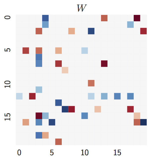

  

• Estimate with n = 1000 samples: lambda = 0, lambda = 0.1, and FGS (baseline).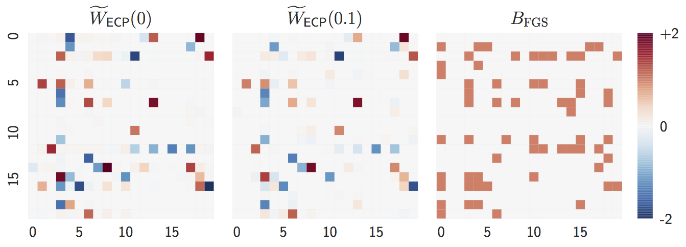

  

  Both lambda = 0 and lambda = 0.1 are close to the ground truth graph when n is large.

• Estimate with n = 20 samples: lambda = 0, lambda = 0.1, and FGS (baseline).

  

  When n is small, lambda = 0 perform worse while lambda = 0.1 remains accurate, showing the advantage of L1-regularization.

• Ground truth: d = 20 nodes, 4d = 80 expected edges.

  

  The degree distribution is significantly different from the Erdos-Renyi graph. One nice property of our method is that it is agnostic about the graph structure.

• Estimate with n = 1000 samples: lambda = 0, lambda = 0.1, and FGS (baseline).

  

  The observation is similar to Erdos-Renyi graph: both lambda = 0 and lambda = 0.1 accurately estimates the ground truth when n is large.

• Estimate with n = 20 samples: lambda = 0, lambda = 0.1, and FGS (baseline).

  

  Similarly, lambda = 0 suffers from small n while lambda = 0.1 remains accurate, showing the advantage of L1-regularization.

• Python: https://github.com/jmoss20/notears
• Tensorflow with Python: https://github.com/ignavier/notears-tensorflow

This is an implementation of the following paper:

[1] Bello K., Aragam B., Ravikumar P. (2022). DAGMA: Learning DAGs via M-matrices and a Log-Determinant Acyclicity Characterization. NeurIPS'22.

If you find this code useful, please consider citing:

@inproceedings{bello2022dagma,
    author = {Bello, Kevin and Aragam, Bryon and Ravikumar, Pradeep},
    booktitle = {Advances in Neural Information Processing Systems},
    title = {{DAGMA: Learning DAGs via M-matrices and a Log-Determinant Acyclicity Characterization}},
    year = {2022}
}

• Summary
  • The log-det acyclicity characterization
  • A path-following approach
• Requirements
• Contents
• Running DAGMA
• Acknowledgments

We propose a new acyclicity characterization of DAGs via a log-det function for learning DAGs from observational data. Similar to previously proposed acyclicity functions (e.g. NOTEARS), our characterization is also exact and differentiable. However, when compared to existing characterizations, our log-det function: (1) Is better at detecting large cycles; (2) Has better-behaved gradients; and (3) Its runtime is in practice about an order of magnitude faster. These advantages of our log-det formulation, together with a path-following scheme, lead to significant improvements in structure accuracy (e.g. SHD).

Let $W \in \mathbb{R}^{d\times d}$ be a weighted adjacency matrix of a graph of $d$ nodes, the log-det function takes the following form:

$$h^{s}(W) = -\log \det (sI-W\circ W) + d \log s,$$

where $I$ is the identity matrix, $s$ is a given scalar (e.g., 1), and $\circ$ denotes the element-wise Hadamard product. Of particular interest, we have that $h(W) = 0$ if and only if $W$ represents a DAG, and when the domain of $h$ is the set of M-matrices then $h$ is well-defined and non-negative. For more properties of $h(W)$ (e.g., being an invex function), $\nabla h(W)$, and $\nabla^2 h(W)$, we invite you to look at [1].

Given the exact differentiable characterization of a DAG, we are interested in solving the following optimization problem:

where $Q$ is a given score function (e.g., square loss) that depends on $W$ and the dataset $\mathbf{X}$. To solve the above constrained problem, we propose a path-following approach where we solve a few of the following unconstrained problems:

where $\mu^{(t)} \to 0$ as $t$ increases. Leveraging the properties of $h$, we show that, at the limit, the solution is a DAG. The trick to make this work is to use the previous solution as a starting point when solving the current unconstrained problem, as usually done in interior-point algorithms. Finally, we use a simple accelerated gradient descent method to solve each unconstrained problem.

Let us give an illustration of how DAGMA works in a two-node graph (see Figure 1 in [1] for more details). Here $w_1$ (the x-axis) represents the edge weight from node 1 to node 2; while $w_2$ (y-axis) represents the edge weight from node 2 to node 1. Moreover, in this example, the ground-truth DAG corresponds to $w_1 = 1.2$ and $w_2 = 0$.

Below we have 4 plots, where each illustrates the solution to an unconstrained problem for different values of $\mu$. In the top-left plot, we have $\mu=1$, and we solve the unconstrained problem starting at the empty graph (i.e., $w_1 = w_2 = 0$), which corresponds to the red point, and after running gradient descent, we arrive at the cyan point (i.e., $w_1 = 1.06, w_2 = 0.24$). Then, for the next unconstrained problem in the top-right plot, we have $\mu = 0.1$, and we initialize gradient descent at the previous solution, i.e., $w_1 = 1.06, w_2 = 0.24$, and arrive at the cyan point $w_1 = 1.16, w_2 = 0.04$. Similarly, DAGMA solves for $\mu=0.01$ and $\mu=0.001$, and we can observe how the solution at the final iteration (bottom-right plot) is close to the ground-truth DAG $w_1 = 1.2, w_2 = 0$.

• Python 3.6+
• numpy
• scipy
• python-igraph
• torch: Only used for nonlinear models.

• dagma_linear.py - implementation of DAGMA for linear models with l1 regularization (supports L2 and Logistic losses).
• dagma_nonlinear.py - implementation of DAGMA for nonlinear models using MLP
• locally_connected.py - special layer structure used for MLP
• utils.py - graph simulation, data simulation, and accuracy evaluation

Use requirements.txt to install the dependencies (recommended to use virtualenv or conda). The simplest way to try out DAGMA is to run a simple example:

$ git clone https://github.com/kevinsbello/dagma.git
$ cd dagma/
$ pip3 install -r requirements.txt
$ python3 dagma_linear.py

The above runs the L1-regularized DAGMA on a randomly generated 20-node Erdos-Renyi graph with 500 samples. Within a few seconds, you should see an output like this:

{'fdr': 0.0, 'tpr': 1.0, 'fpr': 0.0, 'shd': 0, 'nnz': 20}

The data, ground truth graph, and the estimate will be stored in X.csv, W_true.csv, and W_est.csv.

We thank the authors of the NOTEARS repo for making their code available. Part of our code is based on their implementation, specially the utils.py file and some code from their implementation of nonlinear models.

Arkhangelsky, Dmitry, et al. Synthetic difference in differences. No. w25532. National Bureau of Economic Research, 2019. https://www.nber.org/papers/w25532

https://github.com/synth-inference/synthdid

https://medium.com/@masa_asami/causal-inference-using-synthetic-difference-in-differences-with-python-5758e5a76909

$ pip install git+https://github.com/MasaAsami/pysynthdid

This package is still under development. I plan to register with pypi after the following specifications are met.

• Refactoring and better documentation
• Completion of the TEST code

• setup

from synthdid.model import SynthDID
from synthdid.sample_data import fetch_CaliforniaSmoking

df = fetch_CaliforniaSmoking()

PRE_TEREM = [1970, 1988]
POST_TEREM = [1989, 2000]

TREATMENT = ["California"]

• estimation & plot

sdid = SynthDID(df, PRE_TEREM, POST_TEREM, TREATMENT)
sdid.fit(zeta_type="base")
sdid.plot(model="sdid")

• Details of each method will be created later.

• ReproductionExperiment_CaliforniaSmoking.ipynb

  • This is a reproduction experiment note of the original paper, using a famous dataset (CaliforniaSmoking).

• OtherOmegaEstimationMethods.ipynb

  • This note is a different take on the estimation method for parameter omega (& zeta ). As a result, it confirms the robustness of the estimation method in the original paper.

• ScaleTesting_of_DonorPools.ipynb

  • In this note, we will check how the estimation results change with changes in the scale of the donor pool features.
  • Adding donor pools with extremely different scales (e.g., 10x) can have a significant impact (bias) on the estimates.
  • If different scales are mixed, as is usually the case in traditional regression, preprocessing such as logarithmic transformation is likely to be necessary

• This module is still under development.
• If you have any questions or comments, please feel free to use issues.

python setup.py sdist bdist_wheel twine upload dist/* hahray 129)