This is the final project for the course, "Introduction to Neurophysics" in National Tsing Hua University. The goal of this project is to study the binocular balance.

Neural networks, the intricate webs of neurons in our brains, are not just conduits for electrical impulses but the very foundation of learning and perception. Among the various mechanisms governing their adaptability, Hebbian learning stands out as a pivotal concept.

In the followings, we will briefly introduce some basic concepts of Hebbian learning, BCM theory and binocular balance.

Hebbian learning, a fundamental concept in neuroscience, is named after Donald Hebb who proposed it in his 1949 book "The Organization of Behavior." It's often summarized by the phrase "neurons that fire together, wire together." This principle suggests that synaptic connections between neurons are strengthened when they are activated simultaneously. Hebbian learning is crucial for understanding how experiences and behaviors can lead to changes in the brain's neural networks. It's a form of synaptic plasticity, playing a key role in learning and memory. This concept has been instrumental in the development of theories about neural network function and is a foundational element in various fields, including computational neuroscience and psychology.

BCM theory, a pivotal concept in neuroscience, extends the principles of Hebbian learning by introducing a dynamic threshold for synaptic plasticity. BCM theory, formulated in the early 1980s, proposes that the strength of synaptic connections is not only determined by simultaneous neuron activations but also influenced by the history of neuronal activity. The BCM model's innovative feature is its variable threshold, which adapts based on the neuron's previous firing patterns, allowing for a more nuanced understanding of learning and memory processes in the brain. This dynamic threshold mechanism is key to explaining both synaptic strengthening (long-term potentiation) and weakening (long-term depression), offering significant insights into neural adaptability and function.

Binocular balance, a critical aspect of our visual system, ensures a unified and coherent visual experience. It integrates distinct images from each eye, harmonizing them for depth perception and spatial awareness. This process is vital for constructing a stable, accurate representation of our three-dimensional world, illustrating the complexity of neural processing in visual perception and the balance between sensory input and neural activity.

The Hebbian learning rule, if applied simplistically to a multiple-input system like the visual cortex, might lead to a dominance of stronger inputs over weaker ones. However, in reality, sensory inputs are not always of equal strength, and the brain must adapt to this imbalance. In extreme cases, such as with a sensory impairment, this can disrupt neural balance.

Consider a bi-sensory system model, we introduce a negative bias to one of sensory while maintaining a neutral bias in the other. The system undergoes three distinct phases:

1. Pre-treatment, where both inputs receive equal random arrays.
2. Treatment, where the input strength to the normal sensory is deliberately reduced.
3. Post-treatment, where the normal sensory input strength is restored, and the learning rate is significantly reduced to simulate aging effects in neural plasticity.

The detailed methods are in bb.ipynb.

We construct another bi-sensory system model. In this bi-sensory system model focusing on binocular deprivation, both sensory inputs are initially unbiased. The model involves five phases:

1. Normal Rearing, where both inputs receive identical arrays.
2. Monocular Deprivation, reducing the input strength to one sensory system.
3. Binocular Deprivation, reducing input strength to both sensory systems.
4. Reverse Suture, restoring the initially reduced input to one sensory.
5. Binocular Recovery, where both systems receive full-strength, unbiased inputs.

The detailed methods are in bd.ipynb.

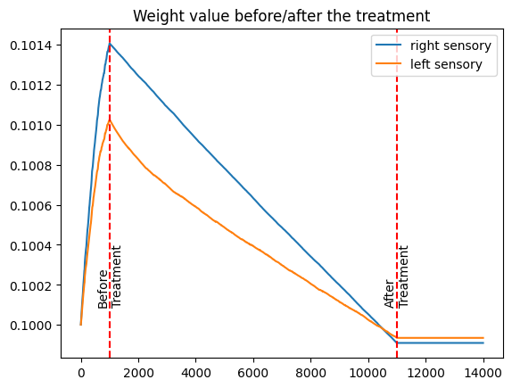
The provided figure illustrates synaptic weight (*average) changes before, during, and after the treatment. Initially, the synaptic weight of the normal sensory input is stronger compared to the amblyopic sensory input. During the treatment phase, we observe a more rapid reduction in the synaptic weight of the normal sensory input. Post-treatment, the synaptic weight of the amblyopic sensory input becomes slightly stronger than that of the normal sensory, achieving a more balanced signal transmission to the cortex.

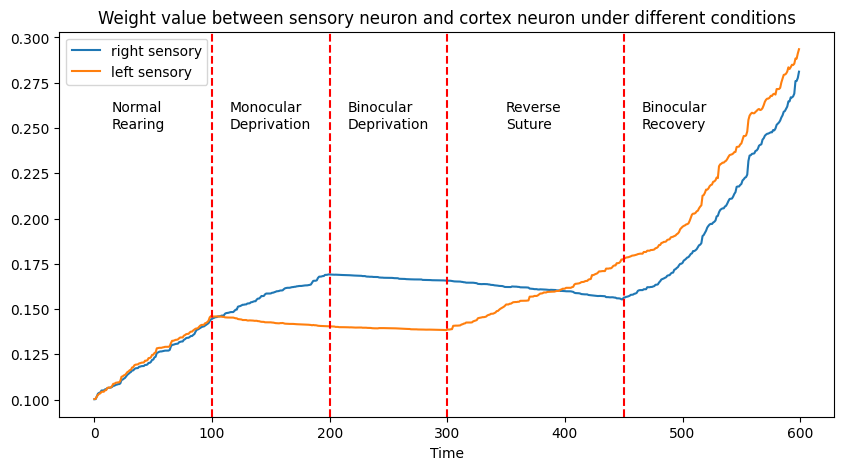
The above figure illustrates synaptic weight changes between the right/left sensory neuron and the cortex neuron under various conditions:

1. Normal Rearing: Equal synaptic weights for both sensory inputs.
2. Monocular Deprivation: Reduced synaptic weight in the deprived sensory neuron.
3. Binocular Deprivation: Slight reduction in synaptic weights for both neurons.
4. Reverse Suture: Restoration of the initially deprived neuron's synaptic weight, coupled with a reduction in the other.
5. Binocular Recovery: An increase in synaptic weights for both neurons.

Comparing these results with real experimental data.

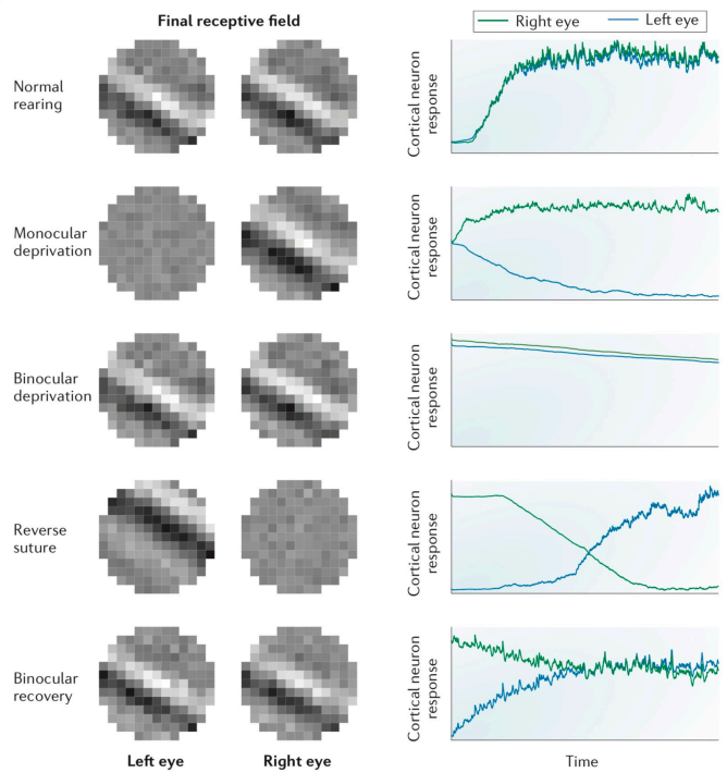
Our model aligns closely except in the final phase, where the actual experiment achieves binocular balance. This discrepancy offers an opportunity for further investigation into the model's parameters or assumptions.

Based on the results, we have following conclusions:

1. Effective amblyopia treatment involves reducing input strength to the normal sensory, demonstrating the adaptability of neural connections.
2. Under typical conditions, binocular balance is naturally achieved through the mechanisms of Hebbian learning and BCM theory.
3. In the case of binocular deprivation, early-age synaptic weight adjustments are feasible due to higher learning rates.
4. Real-world experiments on binocular deprivation show that post-recovery phase synaptic weights can balance out with equal strength inputs, even if initial synaptic weights were imbalanced.

• H.-H. Lin, Handouts in the course, "Introduction to Neurophysics", National Tsing Hua University, 2023.
• W. Gerstner, W. M. Kistler, R. Naud and L. Paninski, "Neuronal Dynamics: From Single Neurons to Networks and Models of Cognition", Cambridge University Press, 2014.