joaquinamatrodrigo / skforecast Goto Github PK
View Code? Open in Web Editor NEWTime series forecasting with scikit-learn models
Home Page: https://skforecast.org
License: BSD 3-Clause "New" or "Revised" License
Time series forecasting with scikit-learn models
Home Page: https://skforecast.org
License: BSD 3-Clause "New" or "Revised" License


Hi,
Is it possible to also predict future values with the implemented SARIMA model? I'm using it as a comparison method based on the backtest predictions and grid_search but not sure if it can also be used to predict into the future (the equivalent to .predict for the autoregressive forecaster).
Thanks
The function backtesting_forecaster() re-train the forecaster with the data included in the argument initial_train_size and overwrite it
Is there a way to get the forecast on training data?
Hi developers,
For better utilizing the multi-series function, I am trying to learn the multi-series deeper by understanding the mechanism based on the case study. However, I still have some confusions about it.
Mechanism: "All series are modeled considering that each time series depends not only on its past values but also on the past values of the other series. The forecaster is expected not only to learn the information of each series separately but also to relate them." Could you explain a little bit more? I tried to read the source codes but I didn't get it after finishing reading the fit() part and got lost.
When I conduct the experiment, I follow the example of the case study and try to change some codes to conduct my own experiments. In the example, results_grid_ms = grid_search_forecaster_multiseries( forecaster = forecaster_ms, series = data.loc[:end_val, :], levels = None, levels_weights = None) and levels and levels_weights is None.
I would like to control the levels and levels_weights to conduct my experiments and follow the API reference, but getting the errors ValueError: "level" must be one of the "series_levels" : ['A','B','C','D'] .
Does it mean that I need to create the for loop like the example of the backtesting_forecaster_multiseries?
`
for i, item in enumerate(data.columns):
metric, preds = backtesting_forecaster_multiseries(
                    forecaster         = forecaster_ms,
                    level              = item,
                    series             = data,
                    steps              = 7,
                )`
change into:
`
for i, item in enumerate(data.columns):
results_grid_ms = grid_search_forecaster_multiseries
                    forecaster         = forecaster_ms,
                    level              = item,  #not sure
                    levels_weights = 1,  # not sure
                    series             = data,
                    steps              = 7,

                )`
However, this method is to "monitor a single model than several". If I create a loop for that, it is not correct to "maintain" the purpose.
results_grid__ms = grid_search_forecaster_multiseries(forecaster = forecaster_ms,series = series) , I create a loop for prediciton:predictions_ms = {} for i, col in enumerate(all_inputs.columns): preds = forecaster_ms.predict(steps=steps,level=col,exog=None) predictions_ms[col] = predshttps://joaquinamatrodrigo.github.io/skforecast/0.4.3/notebooks/forecaster-in-production.html
The note at the end of this page states the following:
It is important to note that last_window's length must be enough to include the maximum lag used by the forecaster. For example, if the forecaster uses lags 1, 24, 48, last_window must include the last 72 values of the series.
I do not understand why would you need 72 values in the above example when your MaxLag is 48?
Hello,
I divided the data into three part: Train, validation and test. I used the backtesting forecaster and predicted the validation data. Then I obtained a rmse via predicted and validation data. Now, I want to predict the test data without giving the test data into the model using backtesting forecaster. I will calculate a rmse again. Then I will forecast the future unknown data.
How can I do that??
Thank you.
It would be nice to be able to test different regressors using grid_search_forecaster.
It could be done by adding a to possibilities to param_grid to be a dict.
In this case, each key would be an instanciated regressor, and values its assiciated param grid search, e.g.:
from sklearn.ensemble import RandomForestRegressor, GradientBoostingRegressor

param_grid = {
    RandomForestRegressor(): {'n_estimators': [50, 100], 'max_depth': [5, 10, 15]},
    GradientBoostingRegressor: {'n_estimators': [50, 100], 'max_depth': [5, 10, 15]}
}It may be useful to five the possibility to decide whether to predict all the models, or just the last one, because sometimes it is required only the last prediction and not all the past ones.
There is a dependency problem with scikit-learn>=1.0 and statsmodels>=0.12, <=0.13, because of scipy's dependency on sckit-learn .Versions of scipy after 1.8.0 have problems with the versions of statsmodels I mentioned as described here. I got the same problem as the stackoverflow post when I tried to import statsmodels.tsa.api.ExponentialSmoothing on my virtual environment after installed skforecast.
from statsmodels.tsa.api import ExponentialSmoothing

>>> ImportError: cannot import name '_centered' from 'scipy.signal.signaltools' (C:\ExamplePath\.venv\lib\site-packages\scipy\signal\signaltools.py)
I ran this on Windows using python 3.9.7
I have split my data into training, validation, and test set. However, while the documentation says in recursive multi-step forecasting, the lagged values came from predicted values (link), and not from the actual values in the test set. I have some doubt from the results of my code:
    outer_start_date = '2017-01-07'
    outer_end_date = '2021-08-21'
    end_train = '2019-06-01'
    end_validation = '2020-07-01'

    selected_forecaster =
    lags_grid = [1, 2, 10, 26, 52, 60, [1, 52]]
    autoregressive_n_lag = 104
    future_prediction_n_step = 8

    forecaster = ForecasterAutoreg(
        regressor=XGBRegressor(random_state=123),
        lags=autoregressive_n_lag  # This value will be replaced in the grid search
    )

    results_grid = grid_search_forecaster(
        forecaster=forecaster,
        y=df.loc[:end_validation, 'REPORTED_CASES'],
        exog=df.loc[:end_validation],
        param_grid=param_grid,
        lags_grid=lags_grid,
        steps=future_prediction_n_step,
        metric=curr_performance_metric,
        refit=refit_in_last_backtest,
        initial_train_size=len(df[:end_train]),
        fixed_train_size=fixed_train_size_in_last_backtest,
        return_best=True,
        verbose=False
    )

    metric, predictions = backtesting_forecaster(
        forecaster=forecaster,
        y=df.REPORTED_CASES,
        initial_train_size=len(df.REPORTED_CASES[:end_validation]),
        fixed_train_size=fixed_train_size_in_last_backtest,
        steps=future_prediction_n_step,
        metric='mean_absolute_error',
        refit=refit_in_last_backtest,
        interval=[5, 95],
        n_boot=500,
        in_sample_residuals=True,
        verbose=False
    )

The model has no features other than the lags based on lags_grid=[1, 2, 10, 26, 52, 60, [1, 52]] . If the assumption is true that lag terms were computed from predicted values in the test set, I shouldn't be seeing this current result that the forecaster seemed to know and matched closely of the drop right before 2020. And we would expect the forecaster to predict a peak in mid/late 2020, which it didn't.
When I changed the lag grid to lags_grid = [[26, 52]], it shows the following which confirms my theory.
Can someone please confirm how lags are chosen during backtesting in the test set? Is there any option I can use the predicted values' lags instead of actual values' lags for the forecasting of the test set values?
Hi,
To be very short:
I tried to fit a lightgbm model onto forecaster and it freezes every time without RAM or memory issues.
Code:
param_grid = {'n_estimators': 2000, 'boosting_type': 'dart', 'max_depth': 45, 'learning_rate': 0.01, 'num_leaves': 25, 'lambda_l1': 0.1, 'lambda_l2': 0.5, 'min_child_samples': 50}

  lags_lightgbm = 16
  forecaster = ForecasterAutoreg(
      regressor=LGBMRegressor(**param_grid), lags=lags_lightgbm
  )
  cols = [col for col in df_to_process_lightgbm.columns if col not in ["ds", "y"]]

  exog = df_to_process_lightgbm[cols]

  forecaster.fit(y=df_to_process_lightgbm["y"], exog=exog) -> here it freezes

  predictions = forecaster.predict(steps=8, exog=exog)

  predictions = predictions.values
Environment: Ubuntu 20.04
certifi                  2022.9.24
charset-normalizer       2.1.1
click                    8.1.3
cliff                    4.1.0
cmaes                    0.9.0
cmd2                     2.4.2
cmdstanpy                1.0.8
colorlog                 6.7.0
comm                     0.1.2
contourpy                1.0.6
convertdate              2.4.0
cycler                   0.11.0
Cython                   0.29.32
debugpy                  1.6.4
decorator                5.1.1
entrypoints              0.4
ephem                    4.1.3
executing                1.2.0
fonttools                4.38.0
frozenlist               1.3.3
greenlet                 2.0.1
hijri-converter          2.2.4
idna                     3.4
importlib-metadata       5.1.0
ipykernel                6.19.2
ipython                  8.7.0
ipywidgets               8.0.3
isoweek                  1.3.3
jedi                     0.18.2
jmespath                 1.0.1
joblib                   1.2.0
kiwisolver               1.4.4
lightgbm                 3.3.3
LunarCalendar            0.0.9
Mako                     1.2.4
MarkupSafe               2.1.1
matplotlib               3.5.0
matplotlib-inline        0.1.6
multidict                6.0.2
mypy-extensions          0.4.3
mysql-connector-python   8.0.31
nest-asyncio             1.5.6
numpy                    1.23.0
nvidia-cublas-cu11       11.10.3.66
nvidia-cuda-nvrtc-cu11   11.7.99
nvidia-cuda-runtime-cu11 11.7.99
nvidia-cudnn-cu11        8.5.0.96
optuna                   2.10.0
packaging                22.0
pandas                   1.4.0
parso                    0.8.3
pathspec                 0.10.2
patsy                    0.5.3
pbr                      5.11.0
pexpect                  4.8.0
pickleshare              0.7.5
Pillow                   9.3.0
pip                      22.3.1
platformdirs             2.6.0
prettytable              3.5.0
prompt-toolkit           3.0.36
protobuf                 3.20.1
psutil                   5.9.4
ptyprocess               0.7.0
pure-eval                0.2.2
pyaml                    21.10.1
Pygments                 2.13.0
PyMeeus                  0.5.12
pyparsing                3.0.9
pyperclip                1.8.2
python-dateutil          2.8.2
python-slugify           6.1.2
pytz                     2022.6
PyYAML                   6.0
pyzmq                    24.0.1
s3transfer               0.6.0
scikit-learn             1.1.0
scikit-optimize          0.9.0
scipy                    1.9.3
seaborn                  0.11.0
setuptools               65.6.3
setuptools-git           1.2
setuptools-scm           7.0.5
six                      1.16.0
skforecast               0.5.1
stack-data               0.6.2
statsmodels              0.13.0
stevedore                4.1.1
tenacity                 8.1.0
text-unidecode           1.3
threadpoolctl            3.1.0
tomli                    2.0.1
torch                    1.12.0
torch-lr-finder          0.2.1
tornado                  6.2
tqdm                     4.64.0
traitlets                5.7.1
typing_extensions        4.4.0
urllib3                  1.26.13
wcwidth                  0.2.5
wheel                    0.38.4
widgetsnbextension       4.0.4
yarl                     1.8.1
Another beginner question - what are the conditions for
refit = True?
I have below error:
d:\programy\miniconda3\lib\site-packages\skforecast\ForecasterAutoreg\ForecasterAutoreg.py in _recursive_predict(self, steps, last_window, exog)
405
406 for i in range(steps):
--> 407 X = last_window[-self.lags].reshape(1, -1)
408 if exog is not None:
409 X = np.column_stack((X, exog[i, ].reshape(1, -1)))
IndexError: index -6 is out of bounds for axis 0 with size 4
If it is important from input side I have following data:
data.shape (50,)
data_train.shape (37,)
data_test.shape (13,)
steps = 13
initial lags: lags = int(data_train.shape[0]*0.4) = 14
whole grid search looks like that:
forecaster_rf = ForecasterAutoreg(
                    regressor = XGBRegressor(verbosity=1),
                    lags = lags
             )
param_grid = {
            'gamma': [0.5, 1, 1.5, 2, 5],
            'subsample': [0.6, 0.8, 1.0],
            'colsample_bytree': [0.6, 0.8, 1.0],
            'max_depth': np.arange(2, 22, 2)
            }

lags_grid = [6, 12, lags, [1, 3, 6, 12, lags]]
below lags throws an error too:
lags_grid = np.arange(1, 3, 1)
lags_grid = [1]
metric = mean_squared_log_error

results_grid = grid_search_forecaster(
                        forecaster         = forecaster_rf,
                        y                  = data_train,
                        param_grid         = param_grid,
                        steps              = steps,
                        metric             = metric,
                        refit              = True,
                        initial_train_size = int(len(data_train)*0.5),
                        return_best        = True,
                        verbose            = True
                   )
Originally posted by @spike8888 in #137 (comment)
Hi,
I am not able to install skforecast in python 3.10 . It seems that statsmodels dependency (>=0.12, <=0.13) does not have a wheel for python 3.10
Hello! :) Nice work thank you!. The method ForecasterAutoreg.create_train_X_y builds the matrix X to feed the regressor calling ForecasterAutoreg.regressor.fit and X is always a pandas DataFrame (except if the regressor is a xgboost). Later, when the ForecasterAutoreg.regressor.predict method is called in a recursive form, each row is a numpy array of shape (1, number_lags + number_exog). This can lead to errors in pipelines that use column transformers because sometimes you need to have the names of the columns to know who to apply the transformations to.
Here is a reproducible example
    import numpy as np
    import pandas as pd
    from sklearn.compose import ColumnTransformer
    from sklearn.pipeline import Pipeline
    from sklearn.preprocessing import MinMaxScaler, OneHotEncoder
    from skforecast.ForecasterAutoreg import ForecasterAutoreg

    lags = 5

    data = pd.Series(
        np.random.rand(100),
        index=pd.date_range("2019-01-01", freq="D", periods=100),
    )
    exog = pd.DataFrame(
        {
            "exog_1": np.random.choice(["A", "B", "C"], len(data)),
            "exog_2": np.random.choice(["D", "E", "F"], len(data)),
        },
        index=data.index,
    )

    preprocessor = ColumnTransformer(
        transformers=[
            (
                "predictors",
                MinMaxScaler(),
                [f"lag_{i}" for i in range(1, lags+ 1)],
            ),
            ("categorical", OneHotEncoder(), ["exog_1", "exog_2"]),
        ],
    )

    pipeline = Pipeline(
        steps=[
            ("preprocessor", preprocessor),
            ("regressor", DecisionTreeRegressor()),
        ],
    )

    forecaster = ForecasterAutoreg(
        lags=lags,
        regressor=pipeline,
    )
    # No problem with fit, every works fine!
    forecaster.fit(data, exog = exog)
    # Here is the problem :(
    forecaster.predict(steps = 1, exog = exog)

 File "~\.venv\lib\site-packages\sklearn\utils\__init__.py", line 353, in _safe_indexing
    raise ValueError(
ValueError: Specifying the columns using strings is only supported for pandas DataFrames
The error occurs as I said, because predict is expecting a pandas DataFrame. A StackOverflow post is here and the example of Column transformer with mixed dtypes is here.
EDIT
Passing the column index instead of its name, works
  preprocessor = ColumnTransformer(
      transformers=[
          (
              "predictors",
              MinMaxScaler(),
              [0,1,2,3,4],
          ),
          ("categorical", OneHotEncoder(), [5,6]),
      ],
  )

  pipeline = Pipeline(
      steps=[
          ("preprocessor", preprocessor),
          ("classifier", DecisionTreeRegressor()),
      ],
  )
I think it would be a good idea to document and/or protect the error inside the code
Hi, this looks pretty similar to sktime, specifically the "reduction" module in forecasting.
https://github.com/alan-turing-institute/sktime
We are currently refactoring that, so would it make sense to work together?
A possible model could be to have interface compatibility, and a "special module" for reduction (direct, recursive, etc)?
Would you like to meet and chat?
The docs say: "ForecasterAutoreg and ForecasterAutoregCustom allow to include exogenous variables as predictors as long as their future values are known, since they must be included during the predict process." source
However, according to the image on the linked website, only the future value of the exogenous variable is included as a predictor, and not its lags. Is there a way to also include the lags of the exogenous variables, not just of the target, in skforecast?
I'm aware that this is possible with a fixed number of lags by using ForecasterAutoregCustom(), but I'm wondering if there is a way to incorporate it into skforecast.model_selection.grid_search_forecaster (in order to not use a fixed number of lags)?
Thanks a lot!
Hello developers,
Would like to consider develop Direct-Recursive hybrid strategies?
TLDR
as the title says, is there a way to pass a verbosity parameter to the fit() function ?
I would love to not have INFOs printed. There are a lot and kinda slow down the code a little bit.
Hello Joaquim,
Couldn´t find how to save the model to a file once is trained, so I can use it later to predict new values.
Is skforecast capable of doing that? and how?
Thank you very much for skforecast! is great!
Hi,
TLDR, because of recent update of setuptools to 65.6.0, could we somehow make this compatible with numpy=1.23.1?
Hi developer,
Since ForecasterAutoregMultiOutput does not contain any API for conducting prediction interval, I try to extract the forecast.regressor and try by myself. However, I realize that if I directly use the regressor to fit(X_train,y_train) and predict(X_train), the result just outputs the condition of fitting without considering the prediction step (for example set step = 6). Because I would like to use the training model residuals to conduct the prediction interval, now the APIs of ForecasterAutoregMultiOutput cannot satisfy my need.
Would you like to provide any suggestion for me to conduct the prediction interval, either in bootstrapping or based on training residuals?
Thank you
Hi developers,
I have a little confusion about using the known exogenous variables to conduct forecasted values.
Firstly, I use the multi-series function to "predict" all the exogenous variables and the target output Y simultaneously. After that, I would like to use the 'predicted values' of the exogenous variables to conduct the direct/recursive forecasting for the target output Y, and I refer the related documents such as the example of weather exogenous variables.
However, I have the confusion about dealing with the known future values in an appropriate place because they are the future known values and the format are "not consistent" with the known training data. How can I "combine" them together during using the skforecast framework?
I am having warning of:
Although the index is: DateTimeIndex, and the frequency is defined as "D"
if I try to replicate ur codes for LGBMRegressor:
import yfinance as yf
import datetime as dt

spxl = yf.Ticker("SPXL")
hist = spxl.history(start="2015-01-01")
hist = hist.asfreq("D")
data = hist.dropna()
type(data.index)
#Output: pandas.core.indexes.datetimes.DatetimeIndex

#Split data into train-val-test
#==============================================================================
data = data.loc['2015-01-01': '2022-12-31']
end_train = '2019-12-31'
end_validation = '2020-12-31'
data_train = data.loc[: end_train, :].copy()
data_val   = data.loc[end_train:end_validation, :].copy()
data_test  = data.loc[end_validation:, :].copy()

#Create forecaster
#==============================================================================
forecaster = ForecasterAutoreg(
                regressor = LGBMRegressor(),
                lags = 7
            )

#Grid search of hyper-parameters and lags
#==============================================================================
#Regressor hyper-parameters
param_grid = {
    'n_estimators': [100, 500],
    'max_depth': [3, 5, 10],
    'learning_rate': [0.01, 0.1]
}

#Lags used as predictors
lags_grid = [7]
results_grid_q10 = grid_search_forecaster(
                            forecaster         = forecaster,
                            y                  = data.loc[:end_validation, 'Close'],
                            param_grid         = param_grid,
                            lags_grid          = lags_grid,
                            steps              = 7,
                            refit              = True,
                            metric             = 'mean_squared_error',
                            initial_train_size = int(len(data_train)),
                            fixed_train_size   = False,
                            return_best        = True,
                            verbose            = False
                    )
I am trying to tune the model using scikit-optimize. But a bunch of errors are coming up. I think it is a good idea to implement bayesian search for this library too.
The functionality of the package is mostly satisfying, but with all due respect, when i compare the performance of skforecast with the model i develop by myself, i found it much slower to use the framework. Once i dive deep into the source code, it comes out that the efficiency problem needs some focus. For example, the _create_lags function may be improved as:
def _create_lags(self, y: np.ndarray) -> Tuple[np.ndarray, np.ndarray]:
    n_splits = len(y) - self.max_lag
    if n_splits <= 0:
        raise Exception(
            "max lag must be less than the length of the series."
        )
    X_data = np.full(shape=(n_splits, len(self.lags)), fill_value=np.nan, dtype=float)

    i = 0
    for lag in self.lags:
        X_data[:, i] = y[self.max_lag - lag: -lag]
        i += 1

    y_data = y[self.max_lag:]
    return X_data, y_data
And i'm sure there is a lot to do about performance optimization, expecting a brand-new version with both satisfying features and speed!
Hi there, recently I have tried skforecast version 0.5.x with _bayesian_optuna_search. In order to make sklearn SVR work properly, I have to add StandardScaler and intend to use Pipeline.
However, after several trials, I cannot implement the pipeline in _bayesian_optuna_search. Are there any solutions?
Hi,
i am using gbt algoritms as base regressor for the forecaster. I am interested in using the early stopping feature of those kind algos. Is it possible?
in the case of HistogramGradientboosting i think is easier becuse the early stopping is configures differently.
Thank you in advance
I am using Skforecast for the first time and I am having trouble forecasting steps which is larger than the number of lags. Below is my sample dataframe with 13 historic values
Python Version: 3.8
skforecast version: 0.4.3
historic_data [2022-01-01 77.0] [2022-01-02 77.0] [2022-01-03 77.0] [2022-01-04 77.0] [2022-01-05 77.0] [2022-01-06 77.0] [2022-01-07 77.0] [2022-01-08 77.0] [2022-01-09 77.0] [2022-01-10 77.0] [2022-01-11 77.0] [2022-01-12 77.0] [2022-01-13 77.0]
Forecaster Object after fitting
ForecasterAutoreg
=================
Regressor: XGBRegressor(base_score=0.5, booster='gbtree', colsample_bylevel=1,
             colsample_bynode=1, colsample_bytree=1, enable_categorical=False,
             gamma=0, gpu_id=-1, importance_type=None,
             interaction_constraints='', learning_rate=0.300000012,
             max_delta_step=0, max_depth=6, min_child_weight=1, missing=nan,
             monotone_constraints='()', n_estimators=100, n_jobs=16,
             num_parallel_tree=1, predictor='auto', random_state=123,
             reg_alpha=0, reg_lambda=1, scale_pos_weight=1, subsample=1,
             tree_method='exact', validate_parameters=1, verbosity=0)
Lags: [ 1  2  3  4  5  6  7  8  9 10 11 12]
Window size: 12
Included exogenous: False
Type of exogenous variable: None
Exogenous variables names: None
Training range: [Timestamp('2022-01-01 00:00:00'), Timestamp('2022-01-13 00:00:00')]
Training index type: DatetimeIndex
Training index frequency: D
Regressor parameters: {'objective': 'reg:squarederror', 'base_score': 0.5, 'booster': 'gbtree', 'colsample_bylevel': 1, 'colsample_bynode': 1, 'colsample_bytree': 1, 'enable_categorical': False, 'gamma': 0, 'gpu_id': -1, 'importance_type': None, 'interaction_constraints': '', 'learning_rate': 0.300000012, 'max_delta_step': 0, 'max_depth': 6, 'min_child_weight': 1, 'missing': nan, 'monotone_constraints': '()', 'n_estimators': 100, 'n_jobs': 16, 'num_parallel_tree': 1, 'predictor': 'auto', 'random_state': 123, 'reg_alpha': 0, 'reg_lambda': 1, 'scale_pos_weight': 1, 'subsample': 1, 'tree_method': 'exact', 'validate_parameters': 1, 'verbosity': 0}
Creation date: 2022-06-10 11:16:13
Last fit date: 2022-06-10 11:16:15
Skforecast version: 0.4.3
Code used for fitting and prediction
forecaster = ForecasterAutoreg(
            regressor=XGBRegressor(random_state=123, verbosity=0),
            lags=12
        )
forecaster.fit(y=historic_data_df.loc[:, 'historic_data'])
predicted = forecaster.predict(steps=6)
Error:
self = =================
ForecasterAutoreg
=================
Regressor: XGBRegressor(base_score=0.5, booster='gbtree', col...1, 'verbosity': 0}
Creation date: 2022-06-10 11:17:54
Last fit date: 2022-06-10 11:17:54
Skforecast version: 0.4.3

steps = 6, last_window = array([77.]), exog = None

    def _recursive_predict(
        self,
        steps: int,
        last_window: np.array,
        exog: np.array
    ) -> pd.Series:
        '''
        Predict n steps ahead. It is an iterative process in which, each prediction,
        is used as a predictor for the next step.

        Parameters
        ----------
        steps : int
            Number of future steps predicted.

        last_window : numpy ndarray
            Values of the series used to create the predictors (lags) need in the
            first iteration of prediction (t + 1).

        exog : numpy ndarray, pandas DataFrame
            Exogenous variable/s included as predictor/s.

        Returns
        -------
        predictions : numpy ndarray
            Predicted values.

        '''

        predictions = np.full(shape=steps, fill_value=np.nan)

        for i in range(steps):
>           X = last_window[-self.lags].reshape(1, -1)
E           IndexError: index -2 is out of bounds for axis 0 with size 1
Hello,
I m using the current df (https://www.kaggle.com/datasets/aramacus/electricity-demand-in-victoria-australia) and when I tried to implement the code used here (https://www.cienciadedatos.net/documentos/py29-forecasting-electricity-power-demand-python.html) I have the following issue :
when I run this code
forecaster = ForecasterAutoreg(
regressor = make_pipeline(StandardScaler(), Ridge(random_state=123)),
lags = 20
)
forecaster.fit(y=data_train.price)
print(forecaster)
The data is at day granularity so i also did
data = data.asfreq('1D')
as you can see below my training frequency/range are not detecting the timestamp format while my format is correct when i run
print(type(data_train.index())
What I am doing wrong?


Many thanks for your input !
I have found a bug in the python code on this page "Recursive multi-step forecasting with exogenous variables".
If exog = data_train[['exog_1', 'exog_2']].values is run directly, it will give this error Exception: "exog" must be "pd.Series" or "pd.DataFrame".
Correction, this should be exog = data_train[['exog_1', 'exog_2']] without the .values since a pandas pd.DataFrame is expected. Please make the correction in the appropriate documentation page and code examples, thanks.
Hi, I was having trouble running backtesting_forecaster, specifically here:
File my_path/.venv/lib/python3.9/site-packages/skforecast/model_selection/model_selection.py:244, in _backtesting_forecaster_verbose(index_values, steps, initial_train_size, folds, remainder, refit, fixed_train_size)
    242 print(f"Data partition in fold: {i}")
    243 if i < folds - 1:
--> 244     print(f"    Training:   {index_values[train_idx_start]} -- {index_values[train_idx_end - 1]}  (n={len(index_values[train_idx_start:train_idx_end])})")
    245     print(f"    Validation: {index_values[last_window_end]} -- {index_values[last_window_end + steps - 1]}  (n={len(index_values[last_window_end:last_window_end + steps])})")
    246 else:

File my_path/.venv/lib/python3.9/site-packages/pandas/core/indexes/base.py:5363, in Index.__getitem__(self, key)
   5360 if is_integer(key) or is_float(key):
   5361     # GH#44051 exclude bool, which would return a 2d ndarray
   5362     key = com.cast_scalar_indexer(key, warn_float=True)
-> 5363     return getitem(key)
   5365 if isinstance(key, slice):
   5366     # This case is separated from the conditional above to avoid
   5367     # pessimization com.is_bool_indexer and ndim checks.
   5368     result = getitem(key)

File my_path/.venv/lib/python3.9/site-packages/pandas/core/arrays/datetimelike.py:358, in DatetimeLikeArrayMixin.__getitem__(self, key)
    350 """
    351 This getitem defers to the underlying array, which by-definition can
    352 only handle list-likes, slices, and integer scalars
    353 """
    354 # Use cast as we know we will get back a DatetimeLikeArray or DTScalar,
    355 # but skip evaluating the Union at runtime for performance
    356 # (see https://github.com/pandas-dev/pandas/pull/44624)
    357 result = cast(
--> 358     "Union[DatetimeLikeArrayT, DTScalarOrNaT]", super().__getitem__(key)
    359 )
    360 if lib.is_scalar(result):
    361     return result

File my_path/.venv/lib/python3.9/site-packages/pandas/core/arrays/_mixins.py:298, in NDArrayBackedExtensionArray.__getitem__(self, key)
    296 key = extract_array(key, extract_numpy=True)  # type: ignore[assignment]
    297 key = check_array_indexer(self, key)
--> 298 result = self._ndarray[key]
    299 if lib.is_scalar(result):
    300     return self._box_func(result)

IndexError: only integers, slices (`:`), ellipsis (`...`), numpy.newaxis (`None`) and integer or boolean arrays are valid indices
After some debugging, it seems initial_train_size , which shoukld be of type int is actually a float, and not an integer.
I could not find where does the assignment take place, nor there were tests to catch it, so my workaround was to check in the code and round(initial_train_size), which is far from ideal.
The call i am using is nearly the same as in documentation
# Backtesting
# ==============================================================================
steps = 36
#n_backtesting = 36*3 # The last 9 years are separated for the backtest

metric, predictions_backtest = backtesting_forecaster(
                                    forecaster         = forecaster,
                                    y                  = data_train[y_col].squeeze(),
                                    exog               = data_train[list_of_x_cols],
                                    initial_train_size = len(data_train[y_col])*0.3,
                                    fixed_train_size   = False,
                                    steps              = steps,
                                    metric             = 'mean_absolute_error',
                                    refit              = True,
                                    verbose            = True
                                )

print(f"Backtest error: {metric}")
and
                regressor = lightGBM.LGBMRegressor(num_leaves=31,
                                                    n_jobs=20, random_state=23,
                                                    #lambda_l1 = 0.25,
                                                    reg_alpha=0.2,
                                                    #max_depth = 15
                                   ),
                lags = 24
             )
Let me know if I can help to fix this.
Cheers
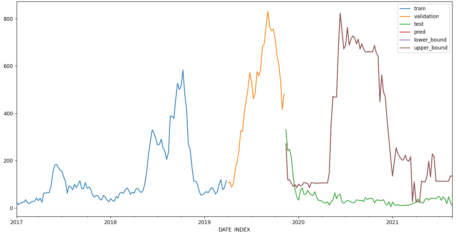
Can someone help explain or point me to how to better interpret these graphs?

I am using XGBRegressor classifier to make prediction in the test period, with each time unit be making a 4-week prediction per step. What can explain the large spikes between Aug and Nov?

Similarly with the prediction interval, what accounts for these large spikes (I set it as interval=[5, 95],), and why the interval only extends above the predicted values?
Edits
The problem space is to predict the number of case count (number of occurrences of an event) in a particular location during the following period. The case count time series (the time unit is weekly) is split into training, validation, and test sets.

Sample data is as follows:
			YEAR  EPIWEEK YEAR_WEEK ADM1_NAME  REPORTED_CASES  BEGINNING    ENDING       DATE \
DATE_INDEX
2017-01-07  2017        1   2017 W          A            89.0   20170101  20170107 2017-01-07
2017-01-14  2017        2   2017 W2         A            84.0   20170108  20170114 2017-01-14
2017-01-21  2017        3   2017 W3         A            87.0   20170115  20170121 2017-01-21
2017-01-28  2017        4   2017 W4         A            51.0   20170122  20170128 2017-01-28
2017-02-04  2017        5   2017 W5         A            41.0   20170129  20170204 2017-02-04

			POPULATION_2020  POPULATION_DENSITY X_AVG_PREC_STD_SCALER  X_AVG_TEMP_STD_SCALER  X_AVG_REL_HUM_STD_SCALER  \
DATE_INDEX
2017-01-07          8348151          106.215978             -0.730876              -1.459063                 -0.661750
2017-01-14          8348151          106.215978             -0.730876              -1.459063                 -0.661750
2017-01-21          8348151          106.215978             -0.730876              -1.459063                 -0.661750
2017-01-28          8348151          106.215978             -0.730876              -1.459063                 -0.661750
2017-02-04          8348151          106.215978             -0.727494              -1.654968                 -0.711259

			X_AVG_SP_HUM_STD_SCALER X_MONTH  X_MA_60    X_MA_30  X_MA_2  X_SMOOTH_MA_2
DATE_INDEX
2017-01-07                -0.960500      01   201.55  97.433333    86.5            NaN
2017-01-14                -0.960500      01   201.55  97.433333    86.5           86.5
2017-01-21                -0.960500      01   201.55  97.433333    85.5           85.5
2017-01-28                -0.960500      01   201.55  97.433333    69.0           69.0
2017-02-04                -1.036021      02   201.55  97.433333    46.0           46.0
The test period is between 2020-07-01 to 2021-08-21. If I make a 4-week rolling prediction (future_prediction_n_step = 4), it looks like this

If I make a 8-week rolling prediction (future_prediction_n_step = 8), it looks like this

My questions are:
My code
import sys
import math
import pandas as pd
import config
import data_import
import feature_engineering as feat_eng
import glob
import numpy as np
import matplotlib.pyplot as plt
import seaborn as sns
import hts
import correlation as corr
from lightgbm import LGBMRegressor
from statsmodels.tsa.stattools import adfuller
from statsmodels.graphics.tsaplots import plot_acf
from statsmodels.graphics.tsaplots import plot_pacf
from sklearn.neighbors import KNeighborsClassifier
from sklearn.preprocessing import StandardScaler
from sklearn.model_selection import train_test_split
from sklearn.linear_model import Ridge, Lasso
from sklearn.ensemble import RandomForestRegressor, GradientBoostingRegressor
from sklearn.pipeline import make_pipeline
from skforecast.ForecasterAutoreg import ForecasterAutoreg
from skforecast.ForecasterAutoregMultiOutput import ForecasterAutoregMultiOutput
from skforecast.model_selection import grid_search_forecaster
from skforecast.model_selection import backtesting_forecaster

# Modelling and Forecasting
# ==============================================================================
from xgboost import XGBRegressor
from lightgbm import LGBMRegressor
from catboost import CatBoostRegressor

from sklearn.preprocessing import OneHotEncoder
from sklearn.preprocessing import StandardScaler
from sklearn.compose import ColumnTransformer
from sklearn.pipeline import make_pipeline

from skforecast.ForecasterAutoreg import ForecasterAutoreg
from skforecast.ForecasterAutoregMultiOutput import ForecasterAutoregMultiOutput
from skforecast.model_selection import grid_search_forecaster
from skforecast.model_selection import backtesting_forecaster

from joblib import dump, load

# Print/graph output setting
save_switch = False  # WARNING: Will overwrite existing files with the same filename
print_switch = True
graph_switch = True
sole_graph_switch = False
if sole_graph_switch:
    graph_switch = False  # if sole_graph_switch == `True`, automatically disable `graph_switch`
prediction_interval_switch = True
log_transform_outcome = False
# Forecasting parameters
autoregressive_n_lag = 104  # number of lags (weeks) used for autoregression
horizontal_threshold_n_case = 100  # this horizontal_threshold_n_case is nullified if set to 0
curr_random_state = 888
lags_grid = [1, 4, 8, 26, 55, 120]   # lags used as autoregressive predictor
curr_performance_metric = 'mean_absolute_error'  # 'mean_absolute_error' # 'mean_squared_error' # 'mean_absolute_percentage_error'
selected_predictor_option_set = 1
param_grid_option = 0  # search grid for hyperparameter optimization
# Moving average setting
slow_ma_n_wk = 60
medium_ma_n_wk = 30
fast_ma_n_wk = 2
smoothing_ma_n_wk = 2
# Date setting
outer_start_date = '2017-01-07'  # '2017-01-07'
outer_end_date = '2021-08-21'  # '2021-08-21'
end_train = '2019-06-01'  # '2019-02-28'
end_validation = '2020-07-01'
restrict_outer_date_switch = True  # if `True`, apply the `outer_start_date` and `outer_end_date` to slice and form the "total" data
# Climate lag setting
avg_precipitation_lag = 0  # positive value, i.e., +4, means the current value will move 4 weeks into the future
avg_temp_lag = 0
avg_relative_humidity_lag = 0
avg_specific_humidity_lag = 0
climate_lag_switch = True  # if `True`, apply the above lags to the corresponding climate var
climate_moving_avg_n_wk = 4
climate_moving_avg_switch = True  # if `True`, turn the climate variables into smooth average


def log_transform(curr_num):
    if curr_num > 0:
        return math.log(curr_num)
    else:
        return curr_num


def main(location, future_prediction_n_step):
    # Setup
    # =====================================================================================================
    # Initial setup
    plt.cla()

    # Data import and preprocessing
    df = data_import.import_single_country_ref_data(input_filename=data_filename)
    df = df.asfreq('W-Sat')  # this line isn't really necessary
    df = df.sort_index()
    assert len(df) > 0, 'Error: DataFrame has no data'

    # Feature set
    # =====================================================================================================
    # Log transformation of outcome (case count)
    if log_transform_outcome:
        df['REPORTED_CASES'] = df['REPORTED_CASES'].apply(log_transform)

    # Data preparation for predictive modeling
    feature_column = ['AVG_PREC', 'AVG_TEMP', 'AVG_REL_HUM', 'AVG_SP_HUM']
    for col in feature_column:
        df.rename(columns={col: 'X_' + col}, inplace=True)  # signal which are predictors

    # Standardize the features
    tagged_feature_column = ['X_AVG_PREC', 'X_AVG_TEMP', 'X_AVG_REL_HUM', 'X_AVG_SP_HUM']
    std_scaler = StandardScaler()
    for col in tagged_feature_column:
        df[col + '_STD_SCALER'] = std_scaler.fit_transform(df[[col]])
    df.drop(tagged_feature_column, axis=1, inplace=True)  # remove unecessary columns

    # Feature engineering - extract month
    df['X_MONTH'] = df['DATE_INDEX_COPY'].dt.strftime('%m')
    df['X_MONTH'] = df['X_MONTH'].astype('category')

    # Feature engineering - moving averages
    df[f'X_MA_{slow_ma_n_wk}'] = df['REPORTED_CASES'].rolling(window=slow_ma_n_wk).mean()
    df[f'X_MA_{medium_ma_n_wk}'] = df['REPORTED_CASES'].rolling(window=medium_ma_n_wk).mean()
    df[f'X_MA_{fast_ma_n_wk}'] = df['REPORTED_CASES'].rolling(window=fast_ma_n_wk).mean()
    df[f'X_SMOOTH_MA_{smoothing_ma_n_wk}'] = df['REPORTED_CASES'].rolling(window=smoothing_ma_n_wk).mean()

    # Feature engineering - case proportion
    df['CASE_PER_100K_POPULATION'] = df[f'X_SMOOTH_MA_{smoothing_ma_n_wk}'] / df['POPULATION_2020'] * 100000

    # Add the REPORTED_CASES time-series (imputed missing) of the adjacent states and map to `df`
    adjacent_adm1_list = config.adjacent_states_per_adm1[location]
    adjacent_adm1_varname_list = []

    for curr_adm1 in adjacent_adm1_list:
        adm1_varname = f'X_REPORTED_CASES_{curr_adm1.upper()}'
        adjacent_adm1_varname_list.append(adm1_varname)
        df_adjacent_adm1 = df_mexico_full[df_mexico_full['ADM1_NAME'] == curr_adm1]
        df_adjacent_adm1 = df_adjacent_adm1[['REPORTED_CASES']]
        df = df.merge(df_adjacent_adm1, left_index=True, right_index=True)
        df.rename({'REPORTED_CASES_y': adm1_varname, 'REPORTED_CASES_x': 'REPORTED_CASES'}, axis=1, inplace=True)

    # Apply lags (in weeks) for climate variables
    if climate_lag_switch:
        df['X_AVG_PREC_STD_SCALER'] = df['X_AVG_PREC_STD_SCALER'].rolling(window=climate_moving_avg_n_wk).mean()
        df['X_AVG_TEMP_STD_SCALER'] = df['X_AVG_TEMP_STD_SCALER'].rolling(window=climate_moving_avg_n_wk).mean()
        df['X_AVG_REL_HUM_STD_SCALER'] = df['X_AVG_REL_HUM_STD_SCALER'].rolling(window=climate_moving_avg_n_wk).mean()
        df['X_AVG_SP_HUM_STD_SCALER'] = df['X_AVG_SP_HUM_STD_SCALER'].rolling(window=climate_moving_avg_n_wk).mean()

    # Predictor groups
    climate_varname_list = ['X_AVG_PREC_STD_SCALER', 'X_AVG_TEMP_STD_SCALER', 'X_AVG_REL_HUM_STD_SCALER',
                            'X_AVG_SP_HUM_STD_SCALER']
    ma_varname_list = [f'X_MA_{slow_ma_n_wk}', f'X_MA_{medium_ma_n_wk}', f'X_MA_{fast_ma_n_wk}']

    # Turn climate variables into their respective moving averages
    if climate_moving_avg_switch:
        df['X_AVG_PREC_STD_SCALER'] = df['X_AVG_PREC_STD_SCALER'].shift(avg_precipitation_lag)
        df['X_AVG_TEMP_STD_SCALER'] = df['X_AVG_TEMP_STD_SCALER'].shift(avg_temp_lag)
        df['X_AVG_REL_HUM_STD_SCALER'] = df['X_AVG_REL_HUM_STD_SCALER'].shift(avg_relative_humidity_lag)
        df['X_AVG_SP_HUM_STD_SCALER'] = df['X_AVG_SP_HUM_STD_SCALER'].shift(avg_specific_humidity_lag)

    # Selection of predictor combinations
    if selected_predictor_option_set == 1:
        exogenous_varname_list = []
    elif selected_predictor_option_set == 2:
        exogenous_varname_list = climate_varname_list
    elif selected_predictor_option_set == 3:
        exogenous_varname_list = adjacent_adm1_varname_list
    elif selected_predictor_option_set == 4:
        exogenous_varname_list = ma_varname_list
    elif selected_predictor_option_set == 5:
        exogenous_varname_list = climate_varname_list + adjacent_adm1_varname_list
    elif selected_predictor_option_set == 6:
        exogenous_varname_list = climate_varname_list + ma_varname_list + adjacent_adm1_varname_list

    # Impute missing values in Exogenous Vars; using last available value
    for varname in (climate_varname_list + ma_varname_list + adjacent_adm1_varname_list):
        df[varname] = df[varname].ffill()  # backward fill - impute using the closest past value
        df[varname] = df[varname].bfill()  # forward fill - inpute using the cloest future value

    # Dataset splitting
    # =====================================================================================================
    # Splitting datasets into train-val-test
    if restrict_outer_date_switch:
        df = df.loc[outer_start_date: outer_end_date]
    df_train = df.loc[: end_train, :]
    df_val = df.loc[end_train:end_validation, :]
    df_test = df.loc[end_validation:, :]

    # Time series plot
    if graph_switch:
        fig, ax = plt.subplots(figsize=(12, 4))
        df_train.REPORTED_CASES.plot(ax=ax, label='train', linewidth=1)
        df_val.REPORTED_CASES.plot(ax=ax, label='validation', linewidth=1)
        df_test.REPORTED_CASES.plot(ax=ax, label='test', linewidth=1)
        ax.set_title(f'Reported cases in {location}')
        ax.legend()

        if log_transform_outcome:
            plt.ylabel('log scale')

        plt.show()

    # Boxplot for annual seasonality
    if graph_switch:
        fig, ax = plt.subplots(figsize=(7, 3.5))
        df['MONTH'] = df.index.month  # WARNING: coarse way to extract month, testing for now
        df.boxplot(column='REPORTED_CASES', by='MONTH', ax=ax, )
        df.groupby('MONTH')['REPORTED_CASES'].median().plot(style='o-', linewidth=0.8, ax=ax)
        ax.set_ylabel('Reported cases')
        ax.set_title(f'Reported cases in {location} by month')
        fig.suptitle('')

        plt.show()

    # Autocorrelation plot
    if graph_switch:
        fig, ax = plt.subplots(figsize=(7, 3))
        plot_acf(df.REPORTED_CASES, ax=ax, lags=180)
        plt.show()

    # Partial autocorrelation plot
    if graph_switch:
        fig, ax = plt.subplots(figsize=(7, 3))
        plot_pacf(df.REPORTED_CASES, ax=ax, lags=112, method='ywm')
        plt.show()

    if print_switch:
        print(f"Train dates : {df_train.index.min()} --- {df_train.index.max()}")
        print(f"Validation dates : {df_val.index.min()} --- {df_val.index.max()}")
        print(f"Test dates : {df_test.index.min()} --- {df_test.index.max()}")
        print(f"Mean outcome: {df['REPORTED_CASES'].mean()}")

    # Forecasting classifier set up (without grid search)
    # =====================================================================================================
    print('=====================================================================================================')
    print('Start of forecasting (without grid search)')

    # Initialize forecaster
    forecaster = ForecasterAutoreg(
        regressor=XGBRegressor(random_state=curr_random_state),
        lags=autoregressive_n_lag
    )

    # Declare predictors and outcome
    forecaster.fit(
        y=df.loc[:end_validation, 'REPORTED_CASES'],
        exog=df.loc[:end_validation, exogenous_varname_list]
    )

    # Backtest
    metric, predictions = backtesting_forecaster(
        forecaster=forecaster,
        y=df.REPORTED_CASES,
        initial_train_size=len(df.loc[:end_validation]),
        fixed_train_size=False,
        steps=future_prediction_n_step,
        metric=curr_performance_metric,
        refit=False,
        verbose=False
    )

    # Plot backtesting and print results
    if graph_switch:
        fig, ax = plt.subplots(figsize=(12, 3.5))
        df.loc[predictions.index, 'REPORTED_CASES'].plot(ax=ax, linewidth=2, label='real')
        predictions.plot(linewidth=2, label='prediction', ax=ax)
        ax.set_title(f'Prediction vs real reported cases in {location} ({future_prediction_n_step}-week)')
        ax.legend()

        if log_transform_outcome:
            plt.ylabel('log scale')

        plt.show()

    if print_switch:
        print(f'Backtest error metric: {metric}')
        print('Predictor importance:', forecaster.get_feature_importance())

    print('End of forecasting (without grid search)')

    # Forecasting classifier set up (with grid search)
    # =====================================================================================================
    print('=====================================================================================================')
    print('Start of forecasting (with grid search)')

    # Hyperparameter Grid search
    forecaster = ForecasterAutoreg(
        regressor=XGBRegressor(random_state=curr_random_state),
        lags=autoregressive_n_lag  # This value will be replaced in the grid search
    )

    # Regressor's hyperparameters
    if param_grid_option == 0:
        param_grid = {
            'n_estimators': [50, 100, 200],
            'max_depth': [5, 10, 30],
            'learning_rate': [0.01, 0.1]
        }

    elif param_grid_option == 1:
        param_grid = {
            'n_estimators': [10, 50, 100, 250, 500],
            'max_depth': [3, 5, 10, 25, 30, 45],
            'learning_rate': [0.01, 0.05, 0.1]
        }

    elif param_grid_option == 2:
        param_grid = {
            'n_estimators': [10, 25, 50, 100, 250, 500, 1000],
            'max_depth': [3, 5, 8, 10, 25, 30, 45],
            'learning_rate': [0.005, 0.01, 0.05, 0.1, 0.3]
        }

    results_grid = grid_search_forecaster(
        forecaster=forecaster,
        y=df.loc[:end_validation, 'REPORTED_CASES'],
        exog=df.loc[:end_validation, exogenous_varname_list],
        param_grid=param_grid,
        lags_grid=lags_grid,
        steps=future_prediction_n_step,
        metric=curr_performance_metric,
        refit=False,
        initial_train_size=len(df[:end_train]),
        fixed_train_size=False,
        return_best=True,
        verbose=False
    )

    if print_switch:
        print(f'Grid optimization results: {results_grid}')
        print(f'Trainer attributes: {forecaster}')

    # Backtest with test data and prediction intervals
    metric, predictions = backtesting_forecaster(
        forecaster=forecaster,
        y=df.REPORTED_CASES,
        initial_train_size=len(df.REPORTED_CASES[:end_validation]),
        fixed_train_size=False,
        steps=future_prediction_n_step,
        metric=curr_performance_metric,
        interval=[5, 95],
        n_boot=500,
        in_sample_residuals=True,
        verbose=False
    )

    if print_switch:
        print('Backtesting error metric:', metric)
        predictions.head(5)

    if graph_switch:
        fig, ax = plt.subplots(figsize=(12, 3.5))
        df.loc[predictions.index, 'REPORTED_CASES'].plot(linewidth=2, label='real', ax=ax)
        ax.set_title(f'Prediction vs real reported cases in {location} ({future_prediction_n_step}-week)')
        predictions.iloc[:, 0].plot(linewidth=2, label='prediction', ax=ax)
        if prediction_interval_switch:
            ax.fill_between(
                predictions.index,
                predictions.iloc[:, 1],
                predictions.iloc[:, 2],
                alpha=0.3,
                color='red',
                label='prediction interval'
            )
        ax.legend()

        if log_transform_outcome:
            plt.ylabel('log scale')

        plt.show()

    if sole_graph_switch:  # mapping the predicted values to the entire time-series
        if prediction_interval_switch:
            fig, ax = plt.subplots(figsize=(18, 6))
            df_train['REPORTED_CASES'].plot(ax=ax, label='train')
            df_val['REPORTED_CASES'].plot(ax=ax, label='validation')
            df_test['REPORTED_CASES'].plot(ax=ax, label='test')
            predictions.plot(ax=ax, label='pred')
            ax.set_title(f'Prediction vs real reported cases in {location} ({future_prediction_n_step}-week)')
            ax.legend()

            if log_transform_outcome:
                plt.ylabel('log scale')

            if save_switch:
                plt.savefig(
                    output_dir + f'/predicted_graph_{location}_{future_prediction_n_step}week_with_interval.png',
                    dpi=300)

            else:
                plt.show()


        else:
            fig, ax = plt.subplots(figsize=(18, 6))
            df_train['REPORTED_CASES'].plot(ax=ax, label='train')
            df_val['REPORTED_CASES'].plot(ax=ax, label='validation')
            df_test['REPORTED_CASES'].plot(ax=ax, label='test')
            predictions.iloc[:, 0].plot(ax=ax, label='pred')
            ax.set_title(f'Prediction vs real reported cases in {location} ({future_prediction_n_step}-week)')
            ax.legend()

            if log_transform_outcome:
                plt.ylabel('log scale')

            if save_switch:
                plt.savefig(output_dir + f'/predicted_graph_{location}_{future_prediction_n_step}week.png', dpi=300)

            else:
                plt.show()

    # Predicted interval coverage
    inside_interval = np.where(
        (df.loc[end_validation:, 'REPORTED_CASES'] >= predictions["lower_bound"]) & \
        (df.loc[end_validation:, 'REPORTED_CASES'] <= predictions["upper_bound"]),
        True,
        False
    )

    coverage = inside_interval.mean()

    if print_switch:
        print(f"Predicted interval coverage: {round(100 * coverage, 2)} %")
        print('Predictor importance:', forecaster.get_feature_importance())


if __name__ == '__main__':
    loop_location_switch = False # can be 'True' or 'False'

    if loop_location_switch == True:
        all_adm1_list = config.adjacent_states_per_adm1.keys()
        n_forecast_week_list = [12, 16, 20, 24, 32, 52]

        for adm1 in all_adm1_list:
            for n_week in n_forecast_week_list:
                main(location=adm1, future_prediction_n_step=n_week)

    else:
        adm1 = config.selected_adm1
        main(location=adm1, future_prediction_n_step=24)
Thanks for the great library! I am trying to apply it to a use case where I need to train a predictor to make a recursive multi-step predictions into the future, where I'd wish to use multiple predicting variables that not related to the target time series itself, but it seems impossible.
First I am aware of the exogenous variables but it requires the future values of exogenous variables are known. In my case, as I need the final forecaster to be able to make multi-steps prediction into future, so this function is not relevant.
For the 'ForecasterAutoregCustom' function where it supports argument of 'fun_predictors', I looked at the source code line 246:
X_train.append(self.create_predictors(y=y_values[train_index]))
It only takes the "y" values as the input but not the other variables that not related to "y". Well, it's very common to have a multi-variate and multi-step forecasting scenario when the future exogenous variables are unknown, I am not quite sure how to do it with this library.
Thank you
Hi !
I'm trying to use your backtesting_forecaster
and when I use and ask for intervals, it leads to ValueError
When no intervals are asked, all works perfectly:
[in]:
if __name__ == "__main__":
    import pandas as pd
    from skforecast.ForecasterAutoreg import ForecasterAutoreg
    from skforecast.model_selection import backtesting_forecaster
    from sklearn.ensemble import RandomForestRegressor

    y_train = pd.Series([479.157, 478.475, 481.205, 492.467, 490.42, 508.166, 523.182,
                         499.634, 495.88, 494.174, 494.174, 490.078, 490.078, 495.539,
                         488.713, 485.3, 493.491, 492.126, 493.832, 485.983, 481.887,
                         474.379, 433.084, 456.633, 477.451, 468.919, 484.959, 471.99,
                         486.324, 498.61, 517.381, 485.3, 480.864, 485.983, 484.276,
                         490.761, 490.078, 494.515, 495.88, 493.15, 491.443, 490.42,
                         485.3, 485.3, 486.665, 467.895, 441.616, 469.601, 477.11,
                         486.324, 485.3, 489.054, 494.856, 513.968, 544.683, 557.31,
                         574.374, 603.383, 617.034, 621.812, 627.273, 612.598, 598.605,
                         610.891, 598.605, 563.112, 542.635, 536.492, 499.634, 456.633,
                         431.037, 453.903, 464.141, 454.244, 456.633, 476.768, 495.88,
                         523.524, 537.516, 577.787, 600.994, 616.693, 631.71, 636.487,
                         621.471, 635.805, 625.908, 616.011, 581.2, 565.842, 553.556,
                         570.279, 514.992, 483.253, 460.046, 469.26, 475.745, 478.816,
                         482.57, 506.801, 510.896])


    backtesting_forecaster(
        forecaster=ForecasterAutoreg(regressor=RandomForestRegressor(random_state=42), lags=10),
        y=y_train,
        steps=24,
        metric="mean_absolute_percentage_error",
        initial_train_size=14,
        n_boot=50,
    )
[out]:
(array([0.07647964]),
           pred
 14   493.40924
 15   493.17717
 16   492.99968
 17   492.98603
 18   492.69932
 ..         ...
 96   492.98603
 97   492.98603
 98   492.98603
 99   492.98603
 100  492.98603

 [87 rows x 1 columns])
however asking for intervals leads to ValueError
[in]:
if __name__ == "__main__":
    import pandas as pd
    from skforecast.ForecasterAutoreg import ForecasterAutoreg
    from skforecast.model_selection import backtesting_forecaster
    from sklearn.ensemble import RandomForestRegressor

    y_train = pd.Series([479.157, 478.475, 481.205, 492.467, 490.42, 508.166, 523.182,
                         499.634, 495.88, 494.174, 494.174, 490.078, 490.078, 495.539,
                         488.713, 485.3, 493.491, 492.126, 493.832, 485.983, 481.887,
                         474.379, 433.084, 456.633, 477.451, 468.919, 484.959, 471.99,
                         486.324, 498.61, 517.381, 485.3, 480.864, 485.983, 484.276,
                         490.761, 490.078, 494.515, 495.88, 493.15, 491.443, 490.42,
                         485.3, 485.3, 486.665, 467.895, 441.616, 469.601, 477.11,
                         486.324, 485.3, 489.054, 494.856, 513.968, 544.683, 557.31,
                         574.374, 603.383, 617.034, 621.812, 627.273, 612.598, 598.605,
                         610.891, 598.605, 563.112, 542.635, 536.492, 499.634, 456.633,
                         431.037, 453.903, 464.141, 454.244, 456.633, 476.768, 495.88,
                         523.524, 537.516, 577.787, 600.994, 616.693, 631.71, 636.487,
                         621.471, 635.805, 625.908, 616.011, 581.2, 565.842, 553.556,
                         570.279, 514.992, 483.253, 460.046, 469.26, 475.745, 478.816,
                         482.57, 506.801, 510.896])


    backtesting_forecaster(
        forecaster=ForecasterAutoreg(regressor=RandomForestRegressor(random_state=42), lags=10),
        y=y_train,
        steps=24,
        metric="mean_absolute_percentage_error",
        initial_train_size=14,
        interval=[95],
        n_boot=50,
    )
[out]:
Traceback (most recent call last):
  File "...\lib\site-packages\IPython\core\interactiveshell.py", line 3398, in run_code
    exec(code_obj, self.user_global_ns, self.user_ns)
  File "<ipython-input-6-9cd2f471a2e7>", line 22, in <cell line: 22>
    backtesting_forecaster(
  File "...\lib\site-packages\skforecast\model_selection\model_selection.py", line 925, in backtesting_forecaster
    metric_value, backtest_predictions = _backtesting_forecaster_no_refit(
  File "...\lib\site-packages\skforecast\model_selection\model_selection.py", line 705, in _backtesting_forecaster_no_refit
    pred = forecaster.predict_interval(
  File "...\lib\site-packages\skforecast\ForecasterAutoreg\ForecasterAutoreg.py", line 757, in predict_interval
    predictions = pd.DataFrame(
  File "...\lib\site-packages\pandas\core\frame.py", line 694, in __init__
    mgr = ndarray_to_mgr(
  File "...\lib\site-packages\pandas\core\internals\construction.py", line 351, in ndarray_to_mgr
    _check_values_indices_shape_match(values, index, columns)
  File "...\dev\lib\site-packages\pandas\core\internals\construction.py", line 422, in _check_values_indices_shape_match
    raise ValueError(f"Shape of passed values is {passed}, indices imply {implied}")
ValueError: Shape of passed values is (24, 2), indices imply (24, 3)Hello
I have a question. Why is the forecast value different even if the last_window data of forecaster.predict and the initial_train_data of backtesting_forecaster are set to be the same period? (using same forecaster)
Did I miss anything?
Hi there, I suggest you to write a short paper and try to publish it, so it is possible to cite your work into other papers throughout google scholar.
I am writing a thesis, is it possible to cite you in any way?
Thank you
Hi developers,
I have a question about fill future known information from one of the exogenous variables.
For example, I have a data where is y as target variable and three exogenous variables X1,X2, and X3. If I have future known information of X3, but no future information of X1,X2. Either using directed or recursive methods, how to integrate the future known exogenous variables (X3) and without future known (X1,X2) and integrate this in the designed framework package?
Hola,
Creo que estás haciendo un gran trabajo con skforecast y los tutoriales que lo acompañan son muy didácticos.
Antes de empezar a usar skforecast la validación cruzada que hago, usando por ejemplo LightGBM, es basarme en TimeSeriesSplit para crear, por ejemplo, 5 particiones, de manera que el proceso de validación cruzada queda más o menos así (la primera columna indica la parte de entrenamiento y la segunda la de validación):
[0,1,2,3,4] [5]
[0,1,2,3,4,5] [6]
[0,1,2,3,4,5,6] [7]
[0,1,2,3,4,5,6,7] [8]
[0,1,2,3,4,5,6,7,8] [9]
En el ejemplo de arriba tendría 5 conjuntos de predicciones validadas y la métrica final sería por ejemplo la media de las métricas obtenidas en cada una de las validaciones. Por tanto, cualquier prueba de selección de modelo estaría sujeta a este bucle de validación cruzada. Al tener 5 particiones o "folds", el modelo habría sido re-entrenado 5 veces lo cual permite usar este bucle de validación cruzada a la hora, por ejemplo, de ajustar hiperparámetros.
Al usar la libreria skforecast, veo que se crea un "fold (para el caso del ForecasterAutoregDirect) del tamaño del número de pasos. En mi caso, esto hace casi siempre inviable el uso de la opción "refit=True", ya que el número de "folds" es muy alto y por tanto se hacen muchos "re-entrenamientos".ç
Por favor, ¿podrías indicarme si hay alguna manera de usar la opción "refit=True" si que haya tantos "re-entrenamientos"?
Un saludo y muchas gracias
Hola, muy bueno tu tutorial de la demanda electrica https://www.cienciadedatos.net/documentos/py29-forecasting-demanda-energia-electrica-python.html
Me gustaria saber cual es la siguiente parte del codigo para ponerlo en produccion, es decir aqui haces las estimaciones hasta la ultima fecha del test 31 diciembre 2014, pero si yo quiero saber la demanda para enero 2015 es decir el futuro, que se deberia hacer.
Pienso que con eso estaria completo el tutorial, gracias por leerle, saludos
Hello! I am new to sk.forecast.ForecasterAutoReg. I tried to implement an LGBM model, and make the predictions on 4 steps ahead. I did manage to visualize the predictions, but I struggle how to plot the curve for the learning part to see how the model performs on the learning dataframe. Below is the code I have used.
`forecaster = ForecasterAutoreg(
regressor=LGBMRegressor(**lgbm_trial_params), lags=[1,2,3,4]
)
cols = [col for col in df.columns if col not in ['date', "Qty"]]
exog = df[cols]
forecaster.fit(y=df["Qty"][:-4], exog=exog[:-4])
predictions = forecaster.predict(steps = 4,exog = exog[:-4])`
Qty represents the target variable I want to predict and my dataframe is structured on weekly data with month, week_num and last_month_average as features.
Here is a printscreen of the structure of my dataframe:

I did not manage to find something useful searching the internet so any help will be much apreciatted. Thanks!
Hi guys.
I was thinking about performing backtesting with overlap in the validation sets. That could be done by having a parameter to define how many periods the forecast origin should advance/shift.
I'll leave an image below that shows the desired backtesting method.
What do you guys think?

Good afternoon!!
When trying to implement :
forecaster = ForecasterAutoreg(
                regressor = XGBRegressor(),
                lags = 24
                )
forecaster
I get the following error:
module 'sklearn' has no attribute 'pipeline'
I looked a lot though internet and somesone said that import sklearn.pipeline would resolve the problem for the moment, but that's not my case... the error remains...
I would be so gratefull if someone helps me!
Thanks a lot
I am trying to apply shap to support vector regression with linear kernel like below:
X_train, y_train = forecaster.create_train_X_y(
y = weightedavg_test['trend'][:-35],
exog = weightedavg_test[['trend_decompose','trend_seasonal','trend_residual','temp_ist','buh_ist','prec_ist' ]][:-35]
)
import shap
shap_values = shap.KernelExplainer(forecaster.predict, X_train).shap_values(X_train)
shap.summary_plot(shap_values,X_train, plot_type="bar")
However, I received an error like that: "The truth value of an array with more than one element is ambiguous. Use a.any() or a.all()". How can I overcome this error?
Originally posted by @yagmurn in #316 (comment)
Hi developers,
The function "get_coef" is deprecated since version 4.3.0, but I would like to use the get_coef with an older version since it easier to interpret to people without machine learning or statistical knowledge compared to use the "impurity-based feature importance" . However, when I use the function "get_coef" in the older version either 4.2.0 or 4.1.0, the program reports error with "AttributeError: 'ForecasterAutoregMultiOutput' object has no attribute 'get_coef'"
Here is the codes I calls for the function:
coef_ = []
for i,j in zip(range(1,7),pd.date_range(start='2022-01',periods=6,freq='M')):
<space>df = pd.DataFrame()
<space>df['feature'] = model_direct.get_coef(step=i)['feature']
<space>df['coef'] = model_direct.get_coef(step=i)['coef']
<space> df['date'] = pd.to_datetime(j)
<space>coef_.append(df)
Thanks.
@JavierEscobarOrtiz
In the current implementation data index is check to verify if it is of type datetime and has frequency. It could happen that there are missing time stamps. Should we rise a warning?
When trying to install skforecast using pip install skforecast, the install process fails with the following output:
note: This error originates from a subprocess, and is likely not a problem with pip.
ERROR: Failed building wheel for numpy
Failed to build numpy
ERROR: Could not build wheels for numpy, which is required to install pyproject.toml-based projects
[end of output]

note: This error originates from a subprocess, and is likely not a problem with pip.
error: subprocess-exited-with-error

× pip subprocess to install build dependencies did not run successfully.
│ exit code: 1
╰─> See above for output.
Unfortunately, the full output is too large, however this seems to happen when trying to install the build dependencies for statsmodels.
Setup:
MacBook Pro M1
MacOS Monterey 12.6
Python 3.9.13 (main, Oct 5 2022, 11:08:35)
Clang 14.0.0 (clang-1400.0.29.102)
Hi,
is this possible to make a parameter to show/hide this?:
2021-08-13 14:28:00,536 root INFO Number of models to fit: 12
loop lags_grid: 0%| | 0/3 [00:00<?, ?it/s]
loop param_grid: 0%| | 0/4 [00:00<?, ?it/s]
loop param_grid: 25%|██▌ | 1/4 [00:00<00:02, 1.39it/s]
loop param_grid: 50%|█████ | 2/4 [00:02<00:02, 1.11s/it]
loop param_grid: 75%|███████▌ | 3/4 [00:02<00:00, 1.08it/s]
loop param_grid: 100%|██████████| 4/4 [00:04<00:00, 1.09s/it]
2021-08-13 14:28:14,897 root INFO Refitting forecaster using the best found parameters and the whole data set:
lags: [ 1 2 3 4 5 6 7 8 9 10]
params: {'max_depth': 10, 'n_estimators': 50}
Best regards and keep up a good work!
Is it possible to integrate this package with SHAP?
A declarative, efficient, and flexible JavaScript library for building user interfaces.
🖖 Vue.js is a progressive, incrementally-adoptable JavaScript framework for building UI on the web.
TypeScript is a superset of JavaScript that compiles to clean JavaScript output.
An Open Source Machine Learning Framework for Everyone
The Web framework for perfectionists with deadlines.
A PHP framework for web artisans
Bring data to life with SVG, Canvas and HTML. 📊📈🎉
JavaScript (JS) is a lightweight interpreted programming language with first-class functions.
Some thing interesting about web. New door for the world.
A server is a program made to process requests and deliver data to clients.
Machine learning is a way of modeling and interpreting data that allows a piece of software to respond intelligently.
Some thing interesting about visualization, use data art
Some thing interesting about game, make everyone happy.
We are working to build community through open source technology. NB: members must have two-factor auth.
Open source projects and samples from Microsoft.
Google ❤️ Open Source for everyone.
Alibaba Open Source for everyone
Data-Driven Documents codes.
China tencent open source team.