lululxvi / deepxde Goto Github PK

Hello,

I tried to using DeepXDE to solve 2D time-dependent heat equations, i.e.

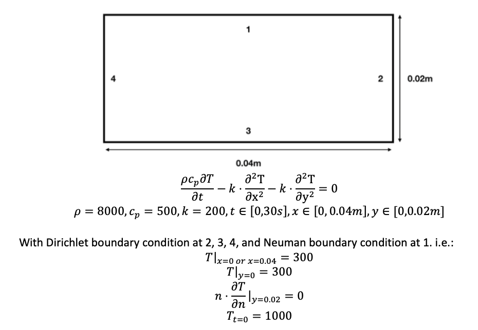
The following is my script:

import numpy as np
import tensorflow as tf
import matplotlib.pyplot as plt
import deepxde as dde
from scipy.interpolate import griddata
import matplotlib.gridspec as gridspec
from mpl_toolkits.mplot3d import axes3d

# geometry parameters
xdim = 200
ydim = 100
xmin = 0.0
ymin = 0.0
xmax = 0.04
ymax = 0.02
# input parameters

rho = 8000
cp = 500
k = 200
T0 = 1000

t0 = 0.0
te = 30.0
x_start = 0.0 # laser start position

# dnn parameters
num_hidden_layer = 3 # number of hidden layers for DNN
hidden_layer_size = 60 # size of each hidden layers
num_domain=1000 # number of training points within domain Tf: random points (spatio-temporal domain)
num_boundary=1000 # number of training boundary condition points on the geometry boundary: Tb
num_initial= 1000 # number of training initial condition points: Tb
num_test=None # number of testing points within domain: uniform generated
epochs=20000 # number of epochs for training
lr=0.001 # learning rate

def main():
    def pde(x, T):
        dT_x = tf.gradients(T, x)[0]
        dT_x, dT_y, dT_t = dT_x[:,0:1], dT_x[:,1:2], dT_x[:,2:]
        dT_xx = tf.gradients(dT_x, x)[0][:, 0:1]
        dT_yy = tf.gradients(dT_y, x)[0][:, 1:2]
        return rho*cp*dT_t -  k*dT_xx - k*dT_yy

    def boundary_x_l(x, on_boundary):
        return on_boundary and np.isclose(x[0], xmin)

    def boundary_x_r(x, on_boundary):
        return on_boundary and np.isclose(x[0], xmax)

    def boundary_y_b(x, on_boundary):
        return on_boundary and np.isclose(x[1], ymin)

    def boundary_y_u(x, on_boundary):
        return on_boundary and np.isclose(x[1], ymax)

    def func(x):
        return np.ones((len(x),1), dtype=np.float32)*T0

    def func_n(x):
        return np.zeros((len(x),1), dtype=np.float32)


    geom = dde.geometry.Rectangle([0, 0], [xmax, ymax])
    timedomain = dde.geometry.TimeDomain(t0, te)
    geomtime = dde.geometry.GeometryXTime(geom, timedomain)

    bc_x_l = dde.DirichletBC(geomtime, func, boundary_x_l)
    bc_x_r = dde.DirichletBC(geomtime, func, boundary_x_r)
    bc_y_b = dde.DirichletBC(geomtime, func, boundary_y_b)
    bc_y_u = dde.NeumannBC(geomtime, func_n, boundary_y_u)
    ic = dde.IC(geomtime, func, lambda _, on_initial: on_initial)

    data = dde.data.TimePDE(
        geomtime,
        pde,
        [bc_x_l, bc_x_r, bc_y_b, bc_y_u, ic],
        num_domain=num_domain,
        num_boundary=num_boundary,
        num_initial=num_initial,
        # train_distribution="uniform",
        num_test=num_test
    )
    net = dde.maps.FNN([3] + [hidden_layer_size] * num_hidden_layer + [1], "tanh", "Glorot uniform")
    model = dde.Model(data, net)

    model.compile("adam", lr=lr)
    losshistory, train_state = model.train(epochs=epochs)
    # model.compile("L-BFGS-B")
    # losshistory, train_state = model.train()
    dde.saveplot(losshistory, train_state, issave=False, isplot=False)

if __name__ == "__main__":
    main()

However, I could not get the converged solution. Basically, the errors on the boundary are not converging. See the following:

Step      Train loss                                                      Test loss                                                       Test metric
0         [1.62e+11, 1.00e+06, 1.00e+06, 1.00e+06, 6.38e-03, 1.00e+06]    [1.62e+11, 0.00e+00, 0.00e+00, 0.00e+00, 0.00e+00, 0.00e+00]    []
1000      [8.22e+05, 9.98e+05, 9.98e+05, 9.98e+05, 9.45e-04, 9.98e+05]    [8.22e+05, 0.00e+00, 0.00e+00, 0.00e+00, 0.00e+00, 0.00e+00]    []
2000      [8.14e+04, 9.96e+05, 9.96e+05, 9.96e+05, 9.77e-04, 9.96e+05]    [8.14e+04, 0.00e+00, 0.00e+00, 0.00e+00, 0.00e+00, 0.00e+00]    []
3000      [4.54e+04, 9.94e+05, 9.94e+05, 9.94e+05, 1.67e-03, 9.94e+05]    [4.54e+04, 0.00e+00, 0.00e+00, 0.00e+00, 0.00e+00, 0.00e+00]    []
4000      [3.79e+04, 9.92e+05, 9.92e+05, 9.92e+05, 1.74e-03, 9.92e+05]    [3.79e+04, 0.00e+00, 0.00e+00, 0.00e+00, 0.00e+00, 0.00e+00]    []
5000      [2.12e+04, 9.91e+05, 9.91e+05, 9.91e+05, 1.76e-03, 9.91e+05]    [2.12e+04, 0.00e+00, 0.00e+00, 0.00e+00, 0.00e+00, 0.00e+00]    []
6000      [1.20e+04, 9.89e+05, 9.89e+05, 9.89e+05, 1.45e-03, 9.89e+05]    [1.20e+04, 0.00e+00, 0.00e+00, 0.00e+00, 0.00e+00, 0.00e+00]    []

Do you have any suggestion how to fix this problem?

Thank you in advance!

I noticed that it will trigger an error if doing arithmetic with TensorFlow tensor, to reproduce

from __future__ import absolute_import
from __future__ import division
from __future__ import print_function

import numpy as np

import deepxde as dde
from deepxde.backend import tf


def main():
    def pde(x, y):
        dy_x = tf.gradients(y, x)[0]
        dy_xx = tf.gradients(dy_x, x)[0]
        return dy_xx - 2

    def boundary_l(x, on_boundary):
        return on_boundary and np.isclose(x[0], -1)

    def boundary_r(x, on_boundary):
        return on_boundary and np.isclose(x[0], 1)

    def func(x):
        return (x + 1) ** 2

    geom = dde.geometry.Interval(-1, 1)
    bc_l = dde.DirichletBC(geom, func, boundary_l)
    bc_r = dde.RobinBC(geom, lambda X, y: tf.math.truediv(y, X), boundary_r)
    data = dde.data.PDE(geom, pde, [bc_l, bc_r], 16, 2, solution=func, num_test=100)

    layer_size = [1] + [50] * 3 + [1]
    activation = "tanh"
    initializer = "Glorot uniform"
    net = dde.maps.FNN(layer_size, activation, initializer)

    model = dde.Model(data, net)
    model.compile("adam", lr=0.001, metrics=["l2 relative error"])
    losshistory, train_state = model.train(epochs=10000)

    dde.saveplot(losshistory, train_state, issave=True, isplot=True)


if __name__ == "__main__":
    main()

the modification is on line 28

    bc_r = dde.RobinBC(geom, lambda X, y: tf.math.truediv(y, X), boundary_r)

the trackback

Traceback (most recent call last):
File "/Library/Frameworks/Python.framework/Versions/3.6/lib/python3.6/contextlib.py", line 99, in exit
self.gen.throw(type, value, traceback)
File "/Users/kyika/.venvs/deepxde/lib/python3.6/site-packages/tensorflow/python/framework/ops.py", line 5652, in get_controller
yield g
File "/Users/kyika/.venvs/deepxde/lib/python3.6/site-packages/tensorflow/python/ops/control_flow_ops.py", line 1977, in cond
orig_res_t, res_t = context_t.BuildCondBranch(true_fn)
File "/Users/kyika/.venvs/deepxde/lib/python3.6/site-packages/tensorflow/python/ops/control_flow_ops.py", line 1814, in BuildCondBranch
original_result = fn()
File "/Users/kyika/Documents/project/pinn/deepxde/deepxde/data/pde.py", line 74, in losses_train
error = bc.error(self.train_x, model.net.inputs, outputs, beg, end)
File "/Users/kyika/Documents/project/pinn/deepxde/deepxde/boundary_conditions.py", line 110, in error
X[beg:end], outputs[beg:end]
File "/Users/kyika/Documents/project/pinn/deepxde/examples/Poisson_Robin_1d.py", line 28, in
bc_r = dde.RobinBC(geom, lambda X, y: tf.math.truediv(y, X), boundary_r)
File "/Users/kyika/.venvs/deepxde/lib/python3.6/site-packages/tensorflow/python/util/dispatch.py", line 180, in wrapper
return target(*args, **kwargs)
File "/Users/kyika/.venvs/deepxde/lib/python3.6/site-packages/tensorflow/python/ops/math_ops.py", line 1051, in truediv
return _truediv_python3(x, y, name)
File "/Users/kyika/.venvs/deepxde/lib/python3.6/site-packages/tensorflow/python/ops/math_ops.py", line 982, in _truediv_python3
(x_dtype, y_dtype))
TypeError: x and y must have the same dtype, got tf.float32 != tf.float64

this probably because the default dtype for NumPy is float64 while TensorFlow is float32, the discrepancy probably introduced from call train_next_batch in deepxde/data/pde.py which generate data using NumPy.

Please have a look at it.

Shunyuan

Hi Lu,

I'm trying to run your newly added euler_beam.py. somehow, it gave me attribute error regarding to a new BC.

"AttributeError: module 'deepxde' has no attribute 'OperatorBC'"

then, I explicitly state this BC as "from deepxde.boundary_conditions import OperatorBC" and it didn't work. after that, I changed "OperatorBC" into "DirichletBC" to do a test run and it worked.

is it possible for you to look into this issue and let me know if I did it wrong by any chance?

much appreciated.
Aaron

Hi Lu, just wondering how can we save network structure and weights after lengthy training so that next time we can only use the pretrained model for predictions rather than starting from scratch (first training then predictions)?

Hi, Lu, thanks for the great work. I try to learn the examples and the code. To start, I modified the lorenz_inverse.py to be forward prolem. However, I cannot get the correct predictions for this simple ode system. I searched your answers to the issues here and tried serveral things, i.e. scale the solution, modified the loss_weight, increase the epochs. Still it is not working. Could you please have a look and tell me how to solve? Many thanks.

from __future__ import absolute_import
from __future__ import division
from __future__ import print_function

import numpy as np
import tensorflow as tf
import matplotlib.pyplot as plt
import deepxde as dde


def gen_traindata():  #get the exp data on t and y1,y2,y3 xzchen
    data = np.load("dataset/Lorenz.npz")#because inverse problem xzchen
    return data["t"], data["y"]


def main():
    C1 = 10. #constant to be estimated 
    C2 = 15.
    C3 = 8./3.

    def Lorenz_system(x, y): #pde system xzchen
        """Lorenz system.
        dy1/dx = 10 * (y2 - y1)
        dy2/dx = y1 * (15- y3) - y2
        dy3/dx = y1 * y2 - 8/3 * y3
        """
        y1, y2, y3 = y[:, 0:1], y[:, 1:2], y[:, 2:]
        dy1_x = tf.gradients(y1, x)[0]
        dy2_x = tf.gradients(y2, x)[0]
        dy3_x = tf.gradients(y3, x)[0]
        return [
            dy1_x - C1 * (y2 - y1),
            dy2_x - y1 * (C2 - y3) + y2,
            dy3_x - y1 * y2 + C3 * y3,
        ]

    def boundary(_, on_initial):
        return on_initial

    geom = dde.geometry.TimeDomain(0, 3) #time start from 0 to 3 

    # Initial conditions
    ic1 = dde.IC(geom, lambda X: -8 * np.ones(X.shape), boundary, component=0)
    ic2 = dde.IC(geom, lambda X: 7 * np.ones(X.shape), boundary, component=1)
    ic3 = dde.IC(geom, lambda X: 27 * np.ones(X.shape), boundary, component=2)

    # Get the train data
    observe_t, ob_y = gen_traindata()

    data = dde.data.PDE(
        geom,
        Lorenz_system,
        [ic1, ic2, ic3],
        num_domain=400,
        num_boundary=10,
        num_test=100,
    )

    net = dde.maps.FNN([1] + [40] * 3 + [3], "tanh", "Glorot uniform")
    #net.outputs_modify(lambda x, y: y * 10) #scale y  

    model = dde.Model(data, net)
    model.compile("adam", lr=0.001)
    #model.compile("adam", lr=0.001,  loss_weights=[1e-1,1e-2,1e-1,1, 1, 1e-1])

    losshistory, train_state = model.train(epochs=60000)
    

    X = geom.uniform_points(100)
    y_pred = model.predict(X)
    #y_dim = y_pred.shape[1]
    S_pred, I_pred, R_pred = y_pred[:, 0:1], y_pred[:, 1:2], y_pred[:, 2:]
    S_ob, I_ob, R_ob = ob_y[:, 0:1], ob_y[:, 1:2], ob_y[:, 2:] 
    plt.figure()
    plt.plot(X, S_pred)
    plt.plot(observe_t, S_ob, "o")    
    plt.plot(X, I_pred)
    plt.plot(X, R_pred)        
    plt.show()
    dde.saveplot(losshistory, train_state, issave=True, isplot=True)


if __name__ == "__main__":
    main()

Hi!
I've seen how you can give weights to the loss on the boundary conditions and the loss on the PDE. But is there also an easy way to give different weights to different residual points in the domain/on the boundary? Or maybe you can tell me where the loss function (equation 2.2 in the paper) is coded?

Hello,
I'd like to ask whether would be possible to add a simple example for Euler equations, even 1D, for example a nozzle flow or 1d shock flow, a riemann problem, please?
Or some hints on how to do it?

Kind regards,
Lorenzo Campoli

Hello,

I am currently trying to implement the Helmholtz equation in 1D (evaluating an acoustical problem) given as:

with a NBC at the left end and a RBC at the right end of the interval.
The value of the NBC equals and the value of the RBC equals
.
In general, the solution given the mentioned BCs is stated as .
Since only the real part is considered, the solution is given as .
The code I used is shown below, but it is not working correctly and I don't know what I did wrong.

# -*- coding: utf-8 -*-
from __future__ import absolute_import
from __future__ import division
from __future__ import print_function

import deepxde as dde
import numpy as np
import tensorflow as tf


def main():
    length = 3.4

    v_s = [-1, 0]  # structural velocity at x=0 and x=length in [m/s]
    rho = 1.3  # fluid density in [kg/m^3]
    c = 340  # speed of sound in [m/s]
    admittance = [0, 1 / (rho * c)]  # boundary admittance at x=0 and x=length in [m^3/(N s)]
    frequency = 200  # frequency in [Hz]
    wavelength = c / frequency  # wavelength in [m]
    k = (2 * np.pi * frequency) / c  # wavenumber in [m^-1]

    def pde(x, y):
        """Helmholtz PDE 1D.

        Parameters
        ----------
        x :
            x-coordinates:
        y :
            Sound pressure solution of Helmholtz PDE.

        Returns
        -------

        """
        dy_x = tf.gradients(y, x)[0]
        dy_xx = tf.gradients(dy_x, x)[0]
        return dy_xx + (k ** 2) * y

    def boundary_left(x, on_boundary):
        """Neumann BC on left boundary.

        Parameters
        ----------
        x
        on_boundary

        Returns
        -------

        """
        return on_boundary and np.isclose(x[0], 0)

    def boundary_right(x, on_boundary):
        """Robin BC on right boundary.

        Parameters
        ----------
        x
        on_boundary

        Returns
        -------

        """
        return on_boundary and np.isclose(x[0], length)

    def func(x):
        """Reference solution real part.

        Parameters
        ----------
        x

        Returns
        -------

        """
        return -v_s[0] * rho * c * np.cos(k * x)

    geom = dde.geometry.Interval(0, length)
    bc_left = dde.NeumannBC(geom, lambda X: v_s[0], boundary_left)
    bc_right = dde.RobinBC(geom, lambda X, y: admittance[1] * y + v_s[1], boundary_right)
    data = dde.data.PDE(geom, pde, [bc_left, bc_right], num_domain=16, num_boundary=2, solution=func, num_test=100)

    layer_size = [1] + [50] * 3 + [1]
    activation = "tanh"
    initializer = "Glorot uniform"
    net = dde.maps.FNN(layer_size, activation, initializer)

    model = dde.Model(data, net)
    model.compile("adam", lr=0.001, metrics=["l2 relative error"])  # metrics=["l2 relative error"]
    losshistory, train_state = model.train(epochs=10000)

    dde.saveplot(losshistory, train_state, issave=False, isplot=True)


if __name__ == "__main__":
    main()

Thank you very much for your help!

dear @lululxvi
I am trying to solve a non-dimensionalized coupled equation of order 1,

but while training the model I am getting several NAN values.

Kindly suggest how to fix it.

coupled eq, domain, BC, code,

and error is as given below:

Error Message:

Code is :

from __future__ import absolute_import
from __future__ import division
from __future__ import print_function


import sys
sys.path.insert( 0, "D:/PhD_Box/Code/Project_1/Stoke_2_DeepXDE/deepxde-master/deepxde-master")

import numpy as np

import deepxde as dde

import tensorflow as tf


def main():

    def pde( x, y ):

        Ra = 1e5
        Pr = 0.71
        pi = 3.14

        u, v, p, T = y[:, 0:1], y[:, 1:2 ], y[:, 2:3], y[:, 3:4]

        du_x = tf.gradients( u , x )[0]
        dv_x = tf.gradients( v , x )[0]
        dp_x = tf.gradients( p , x )[0]
        dT_x = tf.gradients( T , x )[0]


        dp_x, dp_y = dp_x[:, 0:1 ], dp_x[:, 1:2 ]

        du_x, du_y  = du_x[:, 0:1], du_x[:, 1:2 ]

        dv_x, dv_y = dv_x[:, 0:1], dv_x[ :, 1:2 ]

        dT_x, dT_y = dT_x[:, 0:1 ], dT_x[:, 1:2 ]


        du_xx = tf.gradients( du_x, x )[0][:, 0:1 ]
        du_yy = tf.gradients( du_y, x )[0][:, 1:2 ]

        dv_xx = tf.gradients( dv_x, x)[0][:, 0:1 ]
        dv_yy = tf.gradients( dv_y, x)[0][:, 1:2 ]

        dT_xx = tf.gradients( dT_x, x )[0][:, 0:1 ]
        dT_yy = tf.gradients( dT_y, x )[0][:, 1:2 ]



        return [
                du_x + du_y ,
                2*u*du_x + v*du_y+ dp_x - Pr*(du_xx + du_yy),
                du_x*v + u*dv_x + 2*v*dv_y + dp_y - Pr*(dv_xx + dv_yy )+ Ra*Pr*T,
                du_x*T +u*dT_x +dv_y-T + v*dT_y - dT_xx - dT_yy
                ]



    # function definition

    def f_zero(x):

        return np.zeros((len(x),1))

    def f_temp(x):

        pi = 3.14
        return  (1 - np.cos(2*pi*x[:,0:1]))/2


    rect_geom = dde.geometry.Rectangle([0,0], [ 12, 5 ])



    # boundary definition of a unit square domain

    def boundary_left( x, on_boundary ):

        return on_boundary  and np.isclose(x[0], 0 )

    def boundary_right( x, on_boundary ):

        return on_boundary  and np.isclose(x[0], 1 )

    def boundary_upper( x, on_boundary ):

        return on_boundary and np.isclose(x[1], 1 )

    def boundary_lower( x, on_boundary ):

        return on_boundary  and np.isclose(x[1], 0 )


    # defining BC for u, v, and p (component = 0, 1, 2 resp assign)

    bc_left_u = dde.DirichletBC( rect_geom, f_zero, boundary_left, component = 0 )
    bc_left_v = dde.DirichletBC( rect_geom, f_zero , boundary_left, component = 1 )
    bc_left_T = dde.DirichletBC( rect_geom, f_zero , boundary_left, component  = 3)



    bc_right_u = dde.DirichletBC( rect_geom, f_zero, boundary_right, component = 0 )
    bc_right_v = dde.DirichletBC( rect_geom, f_zero , boundary_right, component = 1 )
    bc_right_T = dde.DirichletBC( rect_geom, f_zero , boundary_right, component  = 3)


    bc_lower_u = dde.DirichletBC( rect_geom, f_zero, boundary_lower, component = 0 )
    bc_lower_v = dde.DirichletBC( rect_geom, f_zero, boundary_lower, component = 1 )
    bc_lower_T = dde.DirichletBC( rect_geom, f_temp, boundary_lower, component = 3 )

    bc_upper_u = dde.DirichletBC( rect_geom, f_zero, boundary_upper, component = 0 )
    bc_upper_v = dde.DirichletBC( rect_geom, f_zero, boundary_upper, component = 1 )
    bc_upper_T = dde.DirichletBC(rect_geom, f_zero, boundary_upper, component = 3)


    #bc_lwr_p = dde.DirichletBC(geom, lambda x: 0.00001 * np.ones((len(x), 1)), boundary_upr, component = 2)

    bc = [
             bc_left_u, bc_left_v, bc_left_T,
             bc_right_u, bc_right_v, bc_right_T,
             bc_lower_u, bc_lower_v, bc_lower_T,
             bc_upper_u, bc_upper_v, bc_upper_T,
            ]


    data = dde.data.PDE(
                     rect_geom,
                     pde,
                     bc,
                     num_domain = 1000,
                     num_boundary = 500,
                     num_test = 2000
                   )



    layer_size = [2] + [50] * 2 + [4]
    activation = "tanh"
    initializer = "Glorot uniform"

    net = dde.maps.FNN(layer_size, activation, initializer)

    model = dde.Model(data, net)

    model.compile( "adam", lr = 0.001 )

    losshistory, train_state = model.train(epochs = 5000)

    dde.saveplot(losshistory, train_state, issave=True, isplot=True)


if __name__ == "__main__":
    main()

======================================
Coupled equation and BC are:

• Kindly suggest me for fixing this issue.

Hi,

I'm having trouble using func() when trying to use DeepXDE for a reverse problem.
I have this line: data = dde.data.PDE(geom, 3, odes, [ic1, ic2, ic3, observe_y0, observe_y1, observe_y2], func=func, num_domain=400, num_boundary=2, anchors=observe_t)

And if I leave "func=func" in it, I get this error:
return np.linalg.norm(y_true - y_pred) / np.linalg.norm(y_true) TypeError: unsupported operand type(s) for -: 'NoneType' and 'float'
which occurs upon calling model.train.

However, if I take out the "func=func", because I don't see what it would be used for in this case, I get the error
self.test_y = self.train_y[sum(self.num_bcs) :] if self.train_y else None ValueError: The truth value of an array with more than one element is ambiguous. Use a.any() or a.all()
Which occurs on the line that defines data.

I see in another issue that func is only used to compute test metric, which I don't think I need. So I'd like to not use it.
Would you be able to help me resolve this?

Problem:
After installing tensorflow-gpu in my conda environment, a functional code failed with the following error:

File ".../deepxde/boundary_conditions.py", line 33, in normal_derivative return tf.reduce_sum(dydx * n, axis=1, keepdims=True) TypeError: reduce_sum() got an unexpected keyword argument 'keepdims'

Working fix:
Changing keepdims to keep_dims in the boundary_conditions.py-file seems to fix this issue.

hii @lululxvi ,
I am solving Navier stoke equation which three systems of PDE equation:

while compiling it shows an error for concatenation:

ValueError: all the input array dimensions for the concatenation axis must match exactly, but along dimension 0, the array at index 0 has size 2000 and the array at index 1 has size 1000

Also, in the Geometry part,
I have taken a circle with radius 0.2 centered at the center of rectangle:

Whose code is:

    geom1 = dde.geometry.Rectangle([0,0], [ 12, 5 ])
    geom2 = dde.geometry.Disk( [4.0 , 2.5], 0.2 )
    
    geom = geom1-geom2

I want to put the values of variables over the circle boundary part :
u = 0; (component = 0)
v = 0; ( component =1)

I have coded it as:

bc_circle_u = dde.DirichletBC(geom2, lambda x: np.zeros( (len(x) ,1 ) ), lambda _, on_boundary: on_boundary, component =0)

bc_circle_v = dde.DirichletBC(geom2, lambda x: np.zeros( (len(x) ,1 ) ), lambda _, on_boundary: on_boundary, component =1)

• kindly suggest me whether my code for circle part is right or any modification required:

Dear Lu, great work! I was taking a look at the inverse Lorenz example and I was wondering if it is possible to identify the parameters of the model using only some of the components of the solution (for example the first two components in the Lorenz case) ? Thanks in advance.
Regards
Edie

Hi, I tried to run the Burgers example but I got the error:

  File "D:\wtay\OneDrive\TL\AI_machine_learning\Data\deepxde-master\examples\Burgers.py", line 59, in <module>
    main()

  File "D:\wtay\OneDrive\TL\AI_machine_learning\Data\deepxde-master\examples\Burgers.py", line 39, in main
    geomtime, pde, [bc, ic], num_domain=2540, num_boundary=80, num_initial=160

TypeError: __init__() missing 1 required positional argument: 'ic_bcs'

Any idea what's wrong?

Btw, have you tried using your code on the Navier Stokes eqn? If so, how does it perform? It should be interesting to find out.

Thanks!

Dear @lululxvi

I am trying to implement early stopping over Stoke Equation.

Unfortunately, I am getting an error:

Traceback (most recent call last):

  File "D:\PhD_Box\Code\Project_1\Stoke_DeepXDE\stoke.py", line 179, in <module>
    main()

  File "D:\PhD_Box\Code\Project_1\Stoke_DeepXDE\stoke.py", line 142, in main
    print("Adding new point:", X[x_id], "\n")

IndexError: index 1952 is out of bounds for axis 0 with size 1000

from __future__ import absolute_import
from __future__ import division
from __future__ import print_function

import numpy as np


import sys
sys.path.insert( 0, "D:/PhD_Box/Code/Project_1/Stoke_2_DeepXDE/deepxde-master/deepxde-master")

import deepxde as dde

import tensorflow as tf


def main():

    def pde( x, y ):

        u, v, p = y[:, 0:1], y[:, 1:2 ], y[:, 2:3]

        du_x = tf.gradients( u , x )[0]
        dv_x = tf.gradients( v , x )[0]
        dp_x = tf.gradients( p , x )[0]

        dp_x, dp_y = dp_x[:, 0:1 ], dp_x[:, 1:2 ]

        du_x, du_y = du_x[:, 0:1], du_x[:, 1:2 ]

        dv_x, dv_y = dv_x[:, 0:1], dv_x[ :, 1:2 ]

        du_xx = tf.gradients( du_x, x )[0][:, 0:1 ]
        du_yy = tf.gradients( du_y, x )[0][:, 1:2 ]

        dv_xx = tf.gradients( dv_x, x)[0][:, 0:1 ]
        dv_yy = tf.gradients( dv_y, x)[0][:, 1:2 ]


        return [-( du_xx + du_yy ) + dp_x,
                -( dv_xx + dv_yy ) + dp_y,
                du_x + dv_y ]


    # function definition

    def func(x):

        return np.zeros((len(x),1))

    def func_2(x):

        return np.ones((len(x), 1 ))



    # boundary definition of a unit square domain

    def boundary_l( x, on_boundary ):

        return on_boundary and np.isclose(x[0], 0 )

    def boundary_r( x, on_boundary ):

        return on_boundary and np.isclose(x[0], 1 )

    def boundary_upr( x, on_boundary ):

        return on_boundary and np.isclose(x[1], 1 )

    def boundary_lwr( x, on_boundary ):

        return on_boundary and np.isclose(x[1], 0 )


    geom = dde.geometry.Rectangle([0,0], [ 1, 1 ])


    # defining BC for u, v, and p (component = 0, 1, 2 resp assign)

    bc_lft_u = dde.DirichletBC(geom, func, boundary_l, component = 0 )
    bc_lft_v = dde.DirichletBC(geom, func, boundary_l, component = 1 )

    bc_r_u = dde.DirichletBC(geom, func, boundary_r, component = 0 )
    bc_r_v = dde.DirichletBC(geom, func, boundary_r, component = 1 )

    bc_lwr_u = dde.DirichletBC(geom, func, boundary_lwr, component = 0 )
    bc_lwr_v = dde.DirichletBC(geom, func, boundary_lwr, component = 1 )

    bc_upr_u = dde.DirichletBC(geom, func_2, boundary_upr, component = 0 )
    bc_upr_v = dde.DirichletBC(geom, func, boundary_upr, component = 1 )


    bc_lwr_p = dde.DirichletBC(geom, lambda x: 0.00001 * np.ones((len(x), 1)), boundary_upr, component = 2)



    data = dde.data.PDE(
                     geom,
                     pde,
                     [bc_lft_u, bc_lft_v,
                      bc_r_u, bc_r_v, 
                      bc_lwr_u, bc_lwr_v,
                      bc_upr_u, bc_upr_v,
                      bc_lwr_p ],
                     num_domain = 1000,
                     num_boundary = 500,
                     num_test = 3000
                   )



    layer_size = [2] + [50] * 3 + [3]
    activation = "tanh"
    initializer = "Glorot uniform"

    net = dde.maps.FNN(layer_size, activation, initializer)

    model = dde.Model(data, net)

    model.compile( "adam", lr = 0.001 )

    losshistory, train_state = model.train(epochs = 100)


    
    X = geom.random_points(1000)
    err = 1
    while err > 0.005:
        f = model.predict(X, operator=pde)
        err_eq = np.absolute(f)
        err = np.mean(err_eq)
        print("Mean residual: %.3e" % (err))

        x_id = np.argmax(err_eq)
        print("Adding new point:", X[x_id], "\n")
        data.add_anchors(X[x_id])
        early_stopping = dde.callbacks.EarlyStopping(min_delta=1e-4, patience=2000)
        model.compile("adam", lr=1e-3)
        model.train(
            epochs=10000, disregard_previous_best=True, callbacks=[early_stopping]
        )
        model.compile("L-BFGS-B")
        losshistory, train_state = model.train() 
            
    dde.saveplot(losshistory, train_state, issave=True, isplot=True)
    
    
    #structured linear points
    
    '''x_lin = np.linspace( 0 , 1 , 400 )
    y_lin = np.linspace( 0, 1 , 400 )
    X = np.vstack( ( x_lin, y_lin ) ).T
    y_pred = model.predict( X )
    #y_output_pde = model.predict(X, operator = pde)
    #print( " the dimension of y_pred is:", y_pred.shape )
    #print( " the shape of y_pred by pde is", y_output_pde.shape)
    
    np.savetxt("Linear_prediction.dat", np.hstack((X, y_pred)))
    '''
    x_geom = geom.uniform_points( 5000, boundary = True )
    y_geom_output = model.predict(x_geom)
    
    #print( "the shape of x_geom :", x_geom.shape)
    #print( "the shape of x_geom :", y_geom_output.shape)
    
    np.savetxt( " y_predicted.dat", np.hstack(( x_geom, y_geom_output)) )
    
    
    
    
if __name__ == "__main__":
    main()

Also, I have couple of doubts:

• Why, new points has been deployed over training points.

 print("Adding new point:", X[x_id], "\n")
        data.add_anchors(X[x_id])

• How, can we use the saved trained model for further computation without compiling and investing times again and again.

Kindly, Suggest Thank

In the current master version, it looks like there is a bug in boundary_conditions.py .

I'm solving for multiple components. The error(...) function for DirichletBC checks for values.shape[1] != 1, even though we are allowed to use multiple components and allowed to specify which component the boundary value is for.

Hello Lu,
Can this deep learning library solve this equation?

I'm amazed by your work and as part of a project on PINNs, I would like to test the resolution of inverse problems with DeepXDE. But I'm lost, how do I use DeepXDE for inverse problems where we have to identify functions depending on x, not real parameters? I saw that it was possible thanks to your article "Physics-informed neural networks for inverse problems in nano-optics and metamaterials".
Would it be possible to have an example like in the article with the corresponding code?

Thank you for your reply !

I appreciate the author shares his code with us, faciliating our exploration for PINN. Recently I tried to use the DeepXDE to model the potential flow over cylinder, a brief introduction can be found at https://en.wikipedia.org/wiki/Potential_flow_around_a_circular_cylinder. The governing equation is the Lapace equation in terms of flow potential (phi). I built the geometry using "geom = CSGDifference(rectangular, circle)", and set the Neuman boundary condition using for Rectangular of (u=1, v=0) and Circular(radial velocity of 0, and tangential velocity from analytic solution. The input is two dimensional coordinate and output is one variable(phi). However, when I trained the neural network, the error stuck at 0.1 even if I increased layers/neurons and training steps. None of these attempt succeeds, Hope to get some advice from you.

The code is shown below``` from future import absolute_import
from future import division
from future import print_function

import numpy as np
import tensorflow as tf

import deepxde as dde
from deepxde.geometry.csg import CSGDifference

def main():
def pde(x, phi):
du_xy = tf.gradients(phi, x)[0]
du_x, du_y = du_xy[:, 0:1], du_xy[:, 1:]
du_xx = tf.gradients(du_x, x)[0][:, 0:1]
du_yy = tf.gradients(du_y, x)[0][:, 1:]
return du_xx + du_yy

def Rect_func(x):
    fun = np.concatenate((np.zeros((len(x), 1)) + 1, np.zeros((len(x), 1))), axis=1)
    return fun

U = 1

def Circle_fun(x):
    ux = 2 * U * x[1] ** 2 / (x[0] ** 2 + x[1] ** 2)
    uy = -2 * U * x[1] * x[0] / (x[0] ** 2 + x[1] ** 2)
    Ux = np.expand_dims(ux, axis=0)
    Uy = np.expand_dims(uy, axis=0)

    return np.concatenate((Ux, Uy), axis=1)

circle = dde.geometry.Disk([0, 0], 0.5)
rectangular = dde.geometry.Rectangle([-3, -2], [3, 2])
geom = CSGDifference(rectangular, circle)

def boundary_rect(x, on_boundary):
    return on_boundary and rectangular.on_boundary(x)

def boundary_circle(x, on_boundary):
    return on_boundary and circle.on_boundary(x)

bc_rect = dde.NeumannBC(geom, Rect_func, boundary_rect)
bc_circle = dde.NeumannBC(geom, Circle_fun, boundary_circle)
bcs = [bc_rect, bc_circle]


data = dde.data.PDE(geom, pde, bcs, num_domain=2000, num_boundary=500, num_test=300)
net = dde.maps.FNN([2] + [50] * 5 + [1], "sigmoid", "Glorot uniform")
model = dde.Model(data, net)

model.compile("rmsprop", lr=0.001)
model.train(epochs=6000)
model.compile("L-BFGS-B")
losshistory, train_state = model.train()
dde.saveplot(losshistory, train_state, issave=True, isplot=True)

if name == "main":
main()`

Hey Lu I'd like to understand more about PeriodicBC, what's the PDE problem, specifically the BC for that program ? Also are there other Periodic problems you've seen using DeepXDE ? Thanks !

Hi Lu,

Thank you very much for sharing this amazing tool. I am trying to learn step-by-step process to build PDE and solve it by reviewing examples.

I am trying to write 1D transient diffusion PDE that I have already coded with finite difference method in MATLAB.

dydt = d2ydx2,
Two BCs are : dydx(x=0) = 0 and dydx(x=1) = -2* y
IC : y(t=0) = 1 at all the points.

I have the code here:

def pde(x, y):
    dy_x = tf.gradients(y, x)[0]
    dy_x, dy_t = dy_x[:, 0:1], dy_x[:, 1:]
    dy_xx = tf.gradients(dy_x, x)[0][:, 0:1]
    return dy_t-dy_xx

def boundary_l(x, on_boundary):
    return on_boundary and np.isclose(x[0], 0)

def boundary_r(x, on_boundary):
    return on_boundary and np.isclose(x[0], 1)

geom = dde.geometry.Interval(0, 1)
bc_l = dde.NeumannBC(geom, lambda X: 0 * X, boundary_l)
bc_r = dde.NeumannBC(geom, lambda X: -2 * X, boundary_r)
timedomain = dde.geometry.TimeDomain(0, 1)
geomtime = dde.geometry.GeometryXTime(geom, timedomain)
ic = dde.IC(
    geomtime, lambda x: np.full_like(x[:, 0:1], 1), lambda _, on_initial: on_initial
)
bc = [bc_l, bc_r]
data = dde.data.TimePDE(
    geomtime,
    pde,
    [bc, ic],
    num_domain=400,
    num_boundary=40,
    num_initial=100,
    num_test=10000,
)

layer_size = [2] + [32] * 3 + [1]
activation = "tanh"
initializer = "Glorot uniform"
net = dde.maps.FNN(layer_size, activation, initializer)

model = dde.Model(data, net)

model.compile("adam", lr=0.001, metrics=["l2 relative error"])
losshistory, train_state = model.train(epochs=50000)

dde.saveplot(losshistory, train_state, issave=True, isplot=True)

Currently I am getting error in

data = dde.data.TimePDE(
    geomtime,
    pde,
    [bc, ic],
    num_domain=400,
    num_boundary=40,
    num_initial=100,
    num_test=10000,
)

AttributeError: 'list' object has no attribute 'collocation_points'

I think I did something wrong in bc and ic argument but I am not sure what exactly is wrong. Can you give me some comments on this ? Thank you.

Dear @lululxvi

• Can we add the training point over the domain at a particular position or direction rather than adding it uniformly or randomly over a domain?

for example:

in the case of a square type of domain.

• Only training point should be taken over a line y = x, or a circle type region inside the square geometry.

Hello Lu !

Here's the error log:

     36     geom = dde.geometry.TimeDomain(0, 100)
---> 37     ic1 = dde.IC(geom, lambda X: 1000 * np.ones(X.shape), boundary, component=0)
     38     ic2 = dde.IC(geom, lambda X: 5000 * np.ones(X.shape), boundary, component=1)
     39     ic3 = dde.IC(geom, lambda X: 200 * np.ones(X.shape), boundary, component=2)

AttributeError: 'float' object has no attribute 'ones'

I also get the same error using np.full_like, so I assume the problem is in the component i.e the declared functions in ode_system, what do you think ?
And here's my code:

from __future__ import absolute_import
from __future__ import division
from __future__ import print_function

import numpy as np
import tensorflow as tf

import deepxde as dde
omegap=0.1923
gammap=0.1724
deltap=0.5
kappa=0.5
c=0.5
np=0.0018
mp=0.0018
eps=0.1
bp=3.58
bw=2.30

def main():
    def ode_system(t, y):
        sp, ep, ip,ap,rp,w = y[:, 0:1], y[:, 1:2], y[:, 2:3],y[:, 3:4],y[:, 4:5],y[:, 5:]
        dsp_t = tf.gradients(sp, t)[0]
        dep_t = tf.gradients(ep, t)[0]
        dip_t = tf.gradients(ip, t)[0]
        dap_t = tf.gradients(ap, t)[0]
        drp_t = tf.gradients(rp, t)[0]
        dw_t = tf.gradients(w, t)[0]

        return [
                dsp_t - np + mp * sp + bp * sp * ( ip + kappa * ap ) + bw * sp * w,
                dep_t - bp * sp * ( ip + kappa * ap ) - bw * sp * w + ( 1 - deltap ) * omegap * ep + deltap *  omegap * ep + mp * ep,
                dip_t - ( 1 - deltap ) * omegap * ep + ( gammap + mp ) * ip, 
                dap_t - deltap * omegap * ep + ( gammap + mp ) * ap, 
                drp_t - gammap * ip - gammap * ap + mp * rp,
                dw_t - eps * ( ip + c * ap - w )
                ]

    def boundary(_, on_initial):
        return on_initial

    geom = dde.geometry.TimeDomain(0, 100)
    ic1 = dde.IC(geom, lambda X: 1000 * np.ones(X.shape), boundary, component=0)
    ic2 = dde.IC(geom, lambda X: 5000 * np.ones(X.shape), boundary, component=1)
    ic3 = dde.IC(geom, lambda X: 200 * np.ones(X.shape), boundary, component=2)
    ic4 = dde.IC(geom, lambda X: 800 * np.ones(X.shape), boundary, component=3)
    ic5 = dde.IC(geom, lambda X: 20 * np.ones(X.shape), boundary, component=4)
    ic6 = dde.IC(geom, lambda X: 10 * np.ones(X.shape), boundary, component=5)

    data = dde.data.PDE(
        geom, ode_system, [ic1, ic2, ic3, ic4, ic5, ic6], 1200, 1200, num_test=1500
    )

    layer_size = [1] + [50] * 3 + [6]
    activation = "tanh"
    initializer = "Glorot uniform"
    net = dde.maps.FNN(layer_size, activation, initializer)

    model = dde.Model(data, net)
    model.compile("adam", lr=0.001)
    losshistory, train_state = model.train(epochs=40000)

    dde.saveplot(losshistory, train_state, issave=True, isplot=True)


if __name__ == "__main__":
    main()

I think there may be a bug in the periodic boundary condition. See this test code

from __future__ import absolute_import
from __future__ import division
from __future__ import print_function

import matplotlib.pyplot as plt
import numpy as np
import tensorflow as tf
import sys
import deepxde as dde

def main():
    def pde(x, y):
        dy_x = tf.gradients(y, x)[0]
        dy_x, dy_y = dy_x[:, 0:1], dy_x[:, 1:]
        dy_xx = tf.gradients(dy_x, x)[0][:, 0:1]
        dy_yy = tf.gradients(dy_y, x)[0][:, 1:]

        return -dy_xx-dy_yy-1

    def boundary(x, on_boundary):
        return on_boundary

    def func_bdy(x):
        return np.zeros([len(x), 1])

    def boundary_l(x, on_boundary):
        return on_boundary and np.isclose(x[1], 0)

    def boundary_r(x, on_boundary):
        return on_boundary and np.isclose(x[1], 1.)

    def boundary_t(x, on_boundary):
        return on_boundary and np.isclose(x[0], 1)

    def boundary_b(x, on_boundary):
        return on_boundary and np.isclose(x[0], 0)

    geom = dde.geometry.Rectangle([0,0],[1,1])
    bc = dde.DirichletBC(geom, func_bdy, boundary)

    bc1 = dde.DirichletBC(geom, func_bdy, boundary_l)
    bc2 = dde.DirichletBC(geom, func_bdy, boundary_r)
    bc3 = dde.PeriodicBC(geom, 0, boundary_t)
    #bc4 = dde.PeriodicBC(geom, func_bdy, boundary_b)

    data = dde.data.PDE(
        geom, 1, pde, [bc1, bc2, bc3], num_domain=1200, num_boundary=120, num_test=1500
    )
    metrics_=None
    net = dde.maps.FNN([2] + [50] * 4 + [1], "tanh", "Glorot uniform")
    model = dde.Model(data, net)

    model.compile("adam", lr=0.001, metrics=metrics_)
    model.train(epochs=20000)
    model.compile("L-BFGS-B", metrics=metrics_)
    losshistory, train_state = model.train()
    dde.saveplot(losshistory, train_state, issave=True, isplot=True)

if __name__ == "__main__":
    main()

It is easy to work out that the exact solution is a quadratic function in x. But the results are not.

By looking at a similar issue in https://github.com/lululxvi/deepxde/issues/10, I want to point out the periodic boundary condition is not just u(x, 0)=u(x, 1). In fact, it should be any derivative at both sides are identical. (The formal condition is u(x, y-1)=u(x, y) for any x,y.) There are a few ways to force it. One way has been described in the PINNs paper by Raissi et al.

It is possible that I have a mistake in my code, since I am new to your package. Let me know your suggestion.

Sorry for too many issues, your package has been entertaining us a lot. Thanks a lot for a great package.

Thanks,
Qi

Hi

I would be happy if you could specify the exact versions of dependencies (e.g. tensorflow x.x.x.)? I couldn't see them in the documentation and I am having lots of errors due to depreciated syntax of dependencies. I tried to go ahead and update the source code of the library to the current syntax, but it was just out of control.

Thanks
Yagiz

For example, this happens when running Volterra IDE example:

(deepxde_examples) yagiz@yagiz-ThinkPad-T460s:~/PycharmProjects/deepxde_examples$ python test_libraries.py
Traceback (most recent call last):
File "test_libraries.py", line 64, in
main()
File "test_libraries.py", line 45, in main
net = dde.maps.FNN(layer_size, activation, initializer)
File "/home/yagiz/anaconda3/envs/deepxde_examples/lib/python3.7/site-packages/deepxde/maps/fnn.py", line 32, in init
self.kernel_initializer = initializers.get(kernel_initializer)
File "/home/yagiz/anaconda3/envs/deepxde_examples/lib/python3.7/site-packages/deepxde/maps/initializers.py", line 93, in get
"He normal": tf.variance_scaling_initializer(scale=2.0),
AttributeError: module 'tensorflow' has no attribute 'variance_scaling_initializer'

Hello, I'm having the error in the title using this code

from __future__ import absolute_import
from __future__ import division
from __future__ import print_function

import numpy as np

import deepxde as dde
from deepxde.backend import tf


def main():
    def ode_system(x, y):
        """ODE system.
        dy1/dx = y2
        dy2/dx = -y1
        """
        y1, y2 = y[:, 0:1], y[:, 1:]
        dy1_x = tf.gradients(y1, x)[0]
        dy2_x = tf.gradients(y2, x)[0]
        return [dy1_x + y1*y2*y2, dy2_x - y1*y2*y2]

    def boundary(_, on_initial):
        return on_initial

    geom = dde.geometry.TimeDomain(0, 10)
    ic1 = dde.IC(geom, lambda x: np.full_like(x, 1), boundary, component=0)
    ic2 = dde.IC(geom, lambda x: np.full_like(x, 2), boundary, component=1) 
    data = dde.data.PDE(
        geom, ode_system, [ic1, ic2], 35, 2, num_test=100
    )

    layer_size = [1] + [50] * 3 + [2]
    activation = "tanh"
    initializer = "Glorot uniform"
    net = dde.maps.FNN(layer_size, activation, initializer)

    model = dde.Model(data, net)
    model.compile("adam", lr=0.001, metrics=["l2 relative error"])
    losshistory, train_state = model.train(epochs=20000)

    dde.saveplot(losshistory, train_state, issave=True, isplot=True)


if __name__ == "__main__":
    main()

And further details:

---------------------------------------------------------------------------

TypeError                                 Traceback (most recent call last)

<ipython-input-24-2e2913918ac8> in <module>()
     43 
     44 if __name__ == "__main__":
---> 45     main()

5 frames

<ipython-input-24-2e2913918ac8> in main()
     37     model = dde.Model(data, net)
     38     model.compile("adam", lr=0.001, metrics=["l2 relative error"])
---> 39     losshistory, train_state = model.train(epochs=20000)
     40 
     41     dde.saveplot(losshistory, train_state, issave=True, isplot=True)

/usr/local/lib/python3.6/dist-packages/deepxde/utils.py in wrapper(*args, **kwargs)
     49     def wrapper(*args, **kwargs):
     50         ts = time.time()
---> 51         result = f(*args, **kwargs)
     52         te = time.time()
     53         print("%r took %f s\n" % (f.__name__, te - ts))

/usr/local/lib/python3.6/dist-packages/deepxde/model.py in train(self, epochs, batch_size, display_every, uncertainty, disregard_previous_best, callbacks, model_restore_path, model_save_path, print_model)
    144         self.train_state.set_data_train(*self.data.train_next_batch(self.batch_size))
    145         self.train_state.set_data_test(*self.data.test())
--> 146         self._test(uncertainty)
    147         self.callbacks.on_train_begin()
    148         if train_module.is_scipy_opts(self.optimizer):

/usr/local/lib/python3.6/dist-packages/deepxde/model.py in _test(self, uncertainty)
    291             self.train_state.metrics_test = [
    292                 m(self.train_state.y_test, self.train_state.y_pred_test)
--> 293                 for m in self.metrics
    294             ]
    295 

/usr/local/lib/python3.6/dist-packages/deepxde/model.py in <listcomp>(.0)
    291             self.train_state.metrics_test = [
    292                 m(self.train_state.y_test, self.train_state.y_pred_test)
--> 293                 for m in self.metrics
    294             ]
    295 

/usr/local/lib/python3.6/dist-packages/deepxde/metrics.py in l2_relative_error(y_true, y_pred)
     13 
     14 def l2_relative_error(y_true, y_pred):
---> 15     return np.linalg.norm(y_true - y_pred) / np.linalg.norm(y_true)
     16 
     17 

TypeError: unsupported operand type(s) for -: 'NoneType' and 'float'

when 2 months ago this code

from __future__ import absolute_import
from __future__ import division
from __future__ import print_function

import numpy as np
import tensorflow as tf

import deepxde as dde


def main():
    def ode_system(x, y):
        """ODE system.
        dy1/dx = y2
        dy2/dx = -y1
        """
        u, v = y[:, 0:1], y[:, 1:]
        du_x = tf.gradients(u, x)[0]
        dv_x = tf.gradients(v, x)[0]
        return [du_x + u*v*v, dv_x - u*v*v]

    def boundary(_, on_initial):
        return on_initial 


    geom = dde.geometry.TimeDomain(0,1)
    ic1 = dde.IC(geom, lambda X: 1 * np.ones(X.shape), boundary, component=0)
    ic2 = dde.IC(geom, lambda X: 2 * np.ones(X.shape), boundary, component=1)
    data = dde.data.PDE(geom, 2, ode_system, [ic1, ic2], 35, 2, num_test=100)

    layer_size = [1] + [50] * 3 + [2]
    activation = "tanh"
    initializer = "Glorot uniform"
    net = dde.maps.FNN(layer_size, activation, initializer)

    model = dde.Model(data, net)
    model.compile("adam", lr=0.001, metrics=["l2 relative error"])
    losshistory, train_state = model.train(epochs=20000)

    dde.saveplot(losshistory, train_state, issave=True, isplot=True)


if __name__ == "__main__":
    main()

worked perfectly. What changed ?

System is: {du/dt= -uv^2 ;dv/dt= uv^2; u(0)=1 , v(0)=2}

Thank you !

Hello Lu,

• do you have any example which includes the arbitrary domain used for PDE?

• how to implement the different boundary conditions in a unit circle.
  like upper half-circle include Neumann and lower half-circle include Dirichlet boundary condition.

I got one import module : from deepxde.backend import tf
does it support Tensorflow 2?

Hi Lu,

Thank you for sharing your excellent work!

I am currently working on 2D disk hydrodynamic problem, for example, in Cartesian coordinate system, the domain is x**2+y**2<1, however, since the problem and the boundary condition is more simple under Polar coordinate system (r, theta), one usually want to define the problem in such a coordinate system, as a result, the domain is 0<r<1 && 0<theta<2*pi. In such a case, one need to enforce period boundary condition on theta in order to constrain the problem and get the solution. I am not comfortable with it for these reasons

1. Physically, point (r,theta=0) and point (r,theta=2 pi) is exactly the same point. There is no such thing like a boundary or a step when walking through the "boundary" from 2 pi to 0.
2. Because of the reason above, the physical quantities (and its any order derivative) should strictly equal at theta=2*pi and 0, a soft constraint such as adding sample points and then applying a loss function can not guarantee a strict equal since it is almost impossible to make the loss equal to 0, though it can infinitely close to.
3. Adding one more boundary could make the neural network harder to train.

I noticed that in the work https://doi.org/10.1137/19M1260141, they implemented a method that might could avoid the problem I mentioned above, see last paragraph of 4.3.2

Note that the periodic boundary condition can be strictly imposed by modifying the neural nets unn and Unn by replacing the input x with the combination of sin(2πx/L) and cos(2πx/L), where L is the length of domain D. This is because any continuous 2π-periodic function can be written as a nonlinear function of sin(x) and cos(x). This modification simplifies the loss function by removing the loss due to the periodic boundary condition.

From my point of view, this like adding one additional layer directly after the input layer which map theta to sin(theta) and cos(theta), the point is that:

after the transformation, the neural network can not differentiate 0 and 2 pi, since sin(0)=sin(2 pi) and cos(0)=cos(2 pi).

As a result, no need to sample and enforce period boundary condition.

So I am wondering:

1. What do you think of the problem of periodic boundary condition I mentioned above?
2. What do you think of the method from https://doi.org/10.1137/19M1260141?
3. How to implement the method from https://doi.org/10.1137/19M1260141 in DeepXDE?

Thank you for any help!

Shunyuan

Hi,
I sm wondering whether you have any plan to support TF2 for the deepxde?

As you know, there would be no maintenance of TF1 in the near future.

I want to know about the intermediate steps included for computing PDE using DeepXDE.

• how the forward pass is taking place in DEEPXDE. I mean all collocation points over domain and boundary points have been chosen simultaneously for learning-purpose or only a batch of training points have been chosen.

• Backward pass invoked after completely exhausting the training points or after every single point backward pass has been invoked.

Hello!
I have got an error when using the Euler_beam.py code:

Traceback (most recent call last):
File "", line 53, in
main()
File "", line 43, in main
net = dde.maps.FNN(layer_size, activation, initializer)
File "C:\Users\ThomasFagart\Anaconda3\lib\site-packages\deepxde\maps\fnn.py", line 32, in init
self.kernel_initializer = initializers.get(kernel_initializer)
File "C:\Users\ThomasFagart\Anaconda3\lib\site-packages\deepxde\maps\initializers.py", line 93, in get
"He normal": tf.variance_scaling_initializer(scale=2.0),
AttributeError: module 'tensorflow' has no attribute 'variance_scaling_initializer'

I am using tensorflow 2.0 and python 3.7.3. May that come from the new version of tensorflow?

Thank you very much for your amazing work. Had a few questions.

1. I was able to successfully run it on single GPU but it gave me an OOM error when i increased the domain points to a large value. How do I make it run on a multiple GPU (using TF 1.14). Could you provide me some direction regarding this? Have you ever ran this code on multiple GPU's?

2. After going through the code I believe that currently you have not implemented mini batch. What sort of effort do you think would be required to implement that?

3. Dropouts are used in neural networks in order to prevent overiftting. If we are solving a heat equation then we want the network to learn all the small variations in space and time over the entire domain. Essentially we want to overfit the neural network on that domain to get the most accurate solution so should we use dropouts during training?

Hi
I recently updated the deepxde to 0.5.0 on my macbook. The runs becomes significantly slower. I noticed during the training, the cpu is only limited to around 100%. But it was using 600% previously (using deepxde 0.4.0) I have tensorflow 1.13.

Here is how I install tensorflow and deepxde:

conda create --name tf
conda activate tf
conda install -c conda-forge deepxde

Can you take a look at that? Thanks a lot.

-Qi

Hi Lu,
Thank you very much for sharing this amazing tool. I am trying to use this to solve the Terzaghi equation.
du/dt = Cv*（d2u/dx2）,
Two BCs are : u（0,t）=0,u'(H,t)=0
IC : u(x,0)=1 at all the points.

I want to ask you if my following code is written correctly?

Cv=4.86e-02
H=10

def pde(x, u):
    du_x = tf.gradients(u, x)[0]
    du_x, du_t = du_x[:, 0:1], du_x[:, 1:2]
    du_xx = tf.gradients(du_x, x)[0][:, 0:1]
    return du_t - Cv * du_xx

geom = dde.geometry.Interval(0, H)
timedomain = dde.geometry.TimeDomain(0, 1)
geomtime = dde.geometry.GeometryXTime(geom, timedomain)

def boundary_l(x, on_boundary):
    return on_boundary and np.isclose(x[0], 0)
def boundary_r(x, on_boundary):
    return on_boundary and np.isclose(x[0], H)

bc1 = dde.DirichletBC(
    geomtime, lambda x: np.zeros((len(x), 1)), lambda _, on_boundary: boundary_l
)
bc2 = dde.NeumannBC(
    geomtime, lambda x: np.zeros((len(x), 1)), lambda _, on_boundary: boundary_r
)
ic = dde.IC(
    geomtime, lambda x: np.full_like(x[:, 0:1], 1), lambda _, on_initial: on_initial
)

data = dde.data.TimePDE(
    geomtime, pde, [bc1,bc2,ic], num_domain=2540, num_boundary=80, num_initial=160,num_test=10000
)

net = dde.maps.FNN([2] + [32] * 3 + [1], "tanh", "Glorot normal")
model = dde.Model(data, net)

model.compile("adam", lr=1e-3)
model.train(epochs=50000)
model.compile("L-BFGS-B")
losshistory, train_state = model.train()
dde.saveplot(losshistory, train_state, issave=True, isplot=True)

My final result is strange

Hi, I am interested in solving some practical problems with your solver. As a first test, I would like to solve -div(coeff*grad y) = 1, where coeff=1+x1+x2. (a similar 1D case works fine.) The computational domain is [0,1]^2.

Here is the simple code:

def main():
    def pde(x, y):
        x1=x[:,0]
        x2=x[:,1]
        coeff=1+x1+x2
        dy_x = tf.gradients(y, x)[0]
        dy_x, dy_y = dy_x[:, 0:1], dy_x[:, 1:]
        dy_xx = tf.gradients(coeff*dy_x, x)[0][:, 0:1]
        dy_yy = tf.gradients(coeff*dy_y, x)[0][:, 1:]
        return -dy_xx-dy_yy-1

    def boundary(x, on_boundary):
        return on_boundary

    def func(x):
        return np.zeros([len(x), 1])

    geom = dde.geometry.Rectangle([0,0],[1,1])
    bc = dde.DirichletBC(geom, func, boundary)

    data = dde.data.PDE(
        geom, 1, pde, bc, num_domain=1200, num_boundary=120, num_test=1500
    )
    net = dde.maps.FNN([2] + [50] * 4 + [1], "tanh", "Glorot uniform")
    model = dde.Model(data, net)

    model.compile("adam", lr=0.001)
    model.train(epochs=50000)
    model.compile("L-BFGS-B")
    losshistory, train_state = model.train()
    dde.saveplot(losshistory, train_state, issave=True, isplot=True)

But the solver converges to the wrong solution. One obvious mistake is the boundary condition is not 0 and also the solution is quite off. I also tried the non conserved version of the problem, it give me an even worse solution.

The solver has no issue to solve a problem of -dy_xx-dy_yy-dy_x-dy_y=1, which is very close to the problem I failed. Therefore, I do not quite understand why the solver fails so badly for the problem I set up. I am new to tensorflow, so it is likely I may miss something obvious. Any suggestions?

Thanks!
Qi

from future import absolute_import
from future import division
from future import print_function

import numpy as np

import deepxde as dde

import tensorflow as tf

def main():

def pde(x, y):
    
    phio = 0.1003
    kts = 2.49
    ktf = 0.6
    rhof = 1000
    cpf = 4200
    
    qs = 0
    
    kt = ( 1 - phio )* kts + phio * ktf
    
    
    y1, y2 = y[:, 0:1], y[:, 1:]
    
    y1 = np.zeros(x.shape)
    
    dy2_x = tf.gradients(y2 , x)[0]
    
    dy2_x, dy2_y = dy2_x[:, 0 : 1], dy2_x[:, 1:]
    
    dy2_xx = tf.gradients(dy2_x, x )[0][:, 0:1]
    
    dy2_yy = tf.gradients(dy2_x, x )[0][: , 1:]
    
    return [ y1 , -kt * ( dy2_xx + dy2_yy ) + rhof * cpf * y1 * ( dy2_x + dy2_y) - qs ]
    
    
def func(x):
    
    
    return 473.15 * np.ones(x.shape)
    

def func_n(x):
    
    return np.zeros((x.shape))


geom = dde.geometry.Rectangle([0,0], [10,10])

def boundary_l(x , on_boundary ):
    return on_boundary and np.isclose( x[0], 0 )

def boundary_r(x , on_boundary):
    return on_boundary and np.isclose(x[0], 10)

def boundary_upper(x, on_boundary ):
    return on_boundary and np.isclose(x[1] , 10)

def boundary_lower(x , on_boundary ):
    return on_boundary and np.isclose(x[1], 0)


bc_l = dde.DirichletBC( geom, func, boundary_l )
bc_r = dde.DirichletBC( geom, func, boundary_r )
bc_upper = dde.NeumannBC( geom, func_n, boundary_upper)
bc_lower = dde.NeumannBC( geom, func_n, boundary_lower )


data = dde.data.PDE( geom, pde, [bc_l, bc_r, bc_upper, bc_lower], 
                    num_domain = 1000,
                    num_boundary = 400,
                    num_test = 2500 )

layer_size = [2] + [50]*2 + [2]

activation = "tanh"

initializer = "Glorot uniform"

net = dde.maps.FNN( layer_size, activation, initializer )

model = dde.Model( data, net )
model.compile( "adam", lr = 0.001)
model.train(epochs = 5000 )
model.compile("L-BFGS-B")

losshistory, train_state = model.train()
dde.saveplot(losshistory, train_state, issave=True, isplot=True)

if name == "main":
main()

I am trying to run this code but I am getting error at
y1 = np.zeros(x.shape)

I have replaced it with y1 = np.zeros((len(x),1) also.

error displayed as:
File "D:\PhD_Box\Code\Practice_Code\DEEPXDE\steady.py", line 36, in pde
y1 = np.zeros(x.shape)

TypeError: index returned non-int (type NoneType)

Kindly suggest me how to rectify it.

kindly help me in implementing the different boundary condition in the different geometry of the problem,

Like. in unit square two sides have Dirichlet BC and Two sides have Neumann BC.

while solving simple ODE example [ dy/dx = 0, y(0) =0, domain =[0,1] ]

the solution has a nice agreement with the exact solution but the error value for boundary condition is not equal to zero (approx error at that point is 0.00001).

I think, boundary value are well known for Diff eq, and the error should be equal to zero at that boundary point.

Hello again Lu, sorry for the noobish question but I can only save them as .png.

I use

from google.colab import files
files.download( "train.dat" ) 

And it gives me the .dat file, but did you program anything to do eps and svg ? Or what files are they in ? Or I should just use matlab or python3 to plot the .dat files I have ? Thanks !

When func is provided, my understanding is func is its exact solution, which will be used to compute Test metric. Will it change any other part of the algorithm? Say how test loss is computed?

Solving an electrostatics equation such as
laplacian(phi) = f(x, y, z)
will be easier for the neural network if we are able to supply some engineered inputs such as
1.0/(x^2 + y^2 + z^2)**0.5

Furthermore, suppose we are solving an equation with several interacting electrons which have parameterized positions which could be represented by trainable tf.Variable's:
sum_i 1.0/(x-x_i)**2 + (y-y_i)**2 + (z-z_i)**2

Then, deepxde could be leveraging powerful tools of basis functions as well as neural networks.

Is this currently possible, or can this change be made?

I'm running in a conda env.

Here is the error:

Saving the movie of function to model/movie_x.txt, model/movie_y.txt, model/movie_y.gif...
Traceback (most recent call last):
File "Poisson_Dirichlet_1d.py", line 59, in
main()
File "Poisson_Dirichlet_1d.py", line 43, in main
epochs=10000, callbacks=[checkpointer, movie]
File "//anaconda2/lib/python2.7/site-packages/deepxde/utils.py", line 50, in wrapper
result = f(*args, **kwargs)
File "//anaconda2/lib/python2.7/site-packages/deepxde/model.py", line 119, in train
self.callbacks.on_train_end()
File "//anaconda2/lib/python2.7/site-packages/deepxde/callbacks.py", line 95, in on_train_end
callback.on_train_end()
File "//anaconda2/lib/python2.7/site-packages/deepxde/callbacks.py", line 359, in on_train_end
fname_movie, np.ravel(self.x), self.y, y_reference=y_reference
File "//anaconda2/lib/python2.7/site-packages/deepxde/utils.py", line 105, in save_animation
kwds={"y_reference": y_reference, "logy": logy},
File "//anaconda2/lib/python2.7/site-packages/deepxde/utils.py", line 66, in apply
with Pool(1) as p:
AttributeError: exit

The error does not occur if I comment out the movie and remove movie from the callbacks.

Hello @lululxvi
After training the time evolution problem :

• can we get the intermediate stage of results after training the model?

Hi!
I was analyzing the Poission example for L-shape, but could not figure out how the training data is imported to the model.

Can you please explain how the import of training data works in deepxde? And in which code lines does it happen?

Dear Lu, I have another puzzle when running the code. Let's say we sample 50 points along the boundary, where
bcs = [bc_rectX,bc_rectY, bc_circleX, bc_circleY] data = dde.data.PDE(geom, pde, bcs, num_domain=300, num_boundary=50, num_test=20)
When the code is running, it always issue a warning:
Warning: 50 points required, but 100 points sampled. Uniform random is not guaranteed.
Warning: CSGDifference.uniform_points not implemented. Use random_points instead.

If I set the bounary points=100, it will sample 200 points randomly rather than uniformly. What's the reason causing this problem?

There is a config.py set real=Real(32). Is it true the default precision in deepxde is single precision? If I want to switch to double precision to 64 globally, then I will just do real=Real(64)?

Hello
I was trying to run one of the examples in the DeepXDE, but I encountered this error:

AttributeError: module 'tensorflow' has no attribute 'variance_scaling_initializer'

I have pip installed the latest version of tensorflow and i am running the code in Pycharm.
The thing is when I try to run it in google colab. it will successfully run.

I'll appreciate it if you let me know hat is the problem with running that in Pycharm and Anaconda.

Hey Lu !

I have two questions concerning a system with multiple soltuions (in my case: 6)

1. Is there a way to label them in the plotting ? All I get is the red-dotted graph, but I want to distinguish them. If it's too complicated or long I'd be content enough with just a reference to some plotting documentation that I can follow.
2. After the prediction is done, how can I use the solutions ? Suppose the solutions are (y1,y2,y3,y4,y5,y6), how do I get for example y6(2) ?

Thank you so much, I appreciate your support !

Thank you very much for your work. I'm not ML specialist and I just tried your library for self-education. I met some issues running standard examples.

1. The first problem was that there is no explicit requirement for Python version. I'd like to understand if I have correct version before approaching to installations of any libraries.

2. I found that TensorFlow > v2 isn't working. It produces such error:

AttributeError: module 'tensorflow_core.python.keras.api._v2.keras.losses' has no attribute 'softmax_cross_entropy'

With TensorFlow == 1.15.2 I was able to proceed. Hint: it is good to have versions in your requirements.txt.

3. This problem could be related to Python version.

Traceback (most recent call last):
  File "ode_system.py", line 8, in <module>
    from deepxde.backend import tf
ModuleNotFoundError: No module named 'deepxde.backend'

Actually I don't know why you obfuscate TensorFlow module via your deepxde.backend module. So I got an example working via:

import tensorflow as tf