docs won't deploy

Spatiotemporal Arrays: Raster and Vector Datacubes

Spatiotemporal data often comes in the form of dense arrays, with space and time being array dimensions. Examples include

socio-economic or demographic data,
environmental variables monitored at fixed stations,
raster maps
time series of satellite images with multiple spectral bands,
spatial simulations, and
climate or weather model output.

This R package provides classes and methods for reading, manipulating, plotting and writing such data cubes, to the extent that there are proper formats for doing so.

Raster and vector data cubes

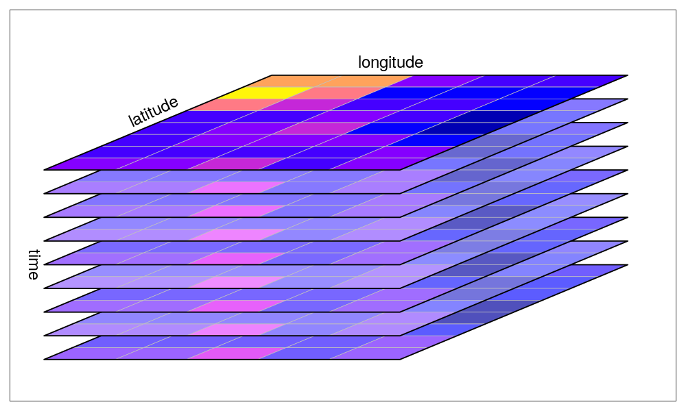
The canonical data cube most of us have in mind is that where two dimensions represent spatial raster dimensions, and the third time (or band), as e.g. shown here:

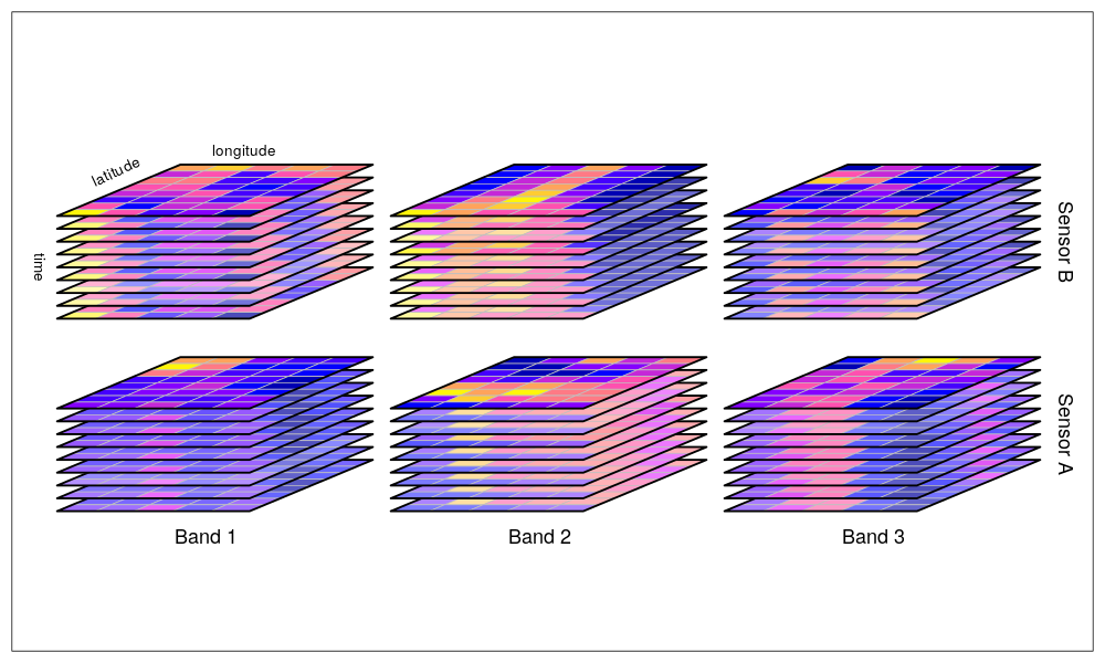
By data cubes however we also consider higher-dimensional cubes (hypercubes) such as a five-dimensional cube where in addition to time, spectral band and sensor form dimensions:

or lower-dimensional cubes such as a raster image:

suppressPackageStartupMessages(library(dplyr))
library(stars)
# Loading required package: abind
# Loading required package: sf
# Linking to GEOS 3.11.2, GDAL 3.7.2, PROJ 9.3.0; sf_use_s2() is TRUE
tif = system.file("tif/L7_ETMs.tif", package = "stars")
read_stars(tif) |>
  slice(index = 1, along = "band") |>
  plot()

Raster data do not need to be regular and aligned with North/East, and package stars supports besides regular also rotated, sheared, rectilinear and curvilinear rasters:

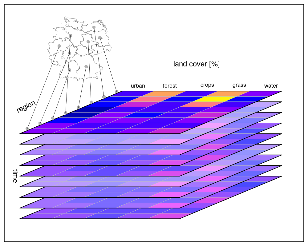
Vector data cubes arise when we do not have two regularly discretized spatial dimensions, but a single dimension that points to distinct spatial feature geometries, such as polygons (e.g. denoting administrative regions):

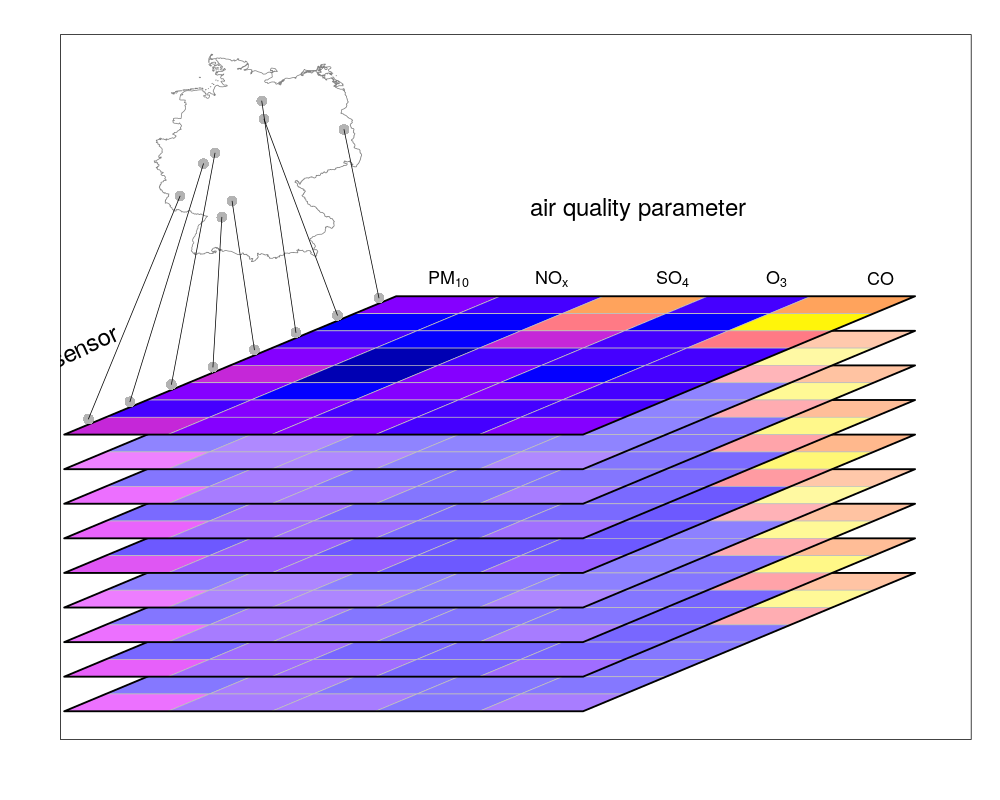
or points (e.g. denoting sensor locations):

NetCDF’s CF-convention calls this a discrete axis.

NetCDF, GDAL

stars provides two functions to read data: read_ncdf and read_stars, where the latter reads through GDAL. (In the future, both will be integrated in read_stars.) For reading NetCDF files, package RNetCDF is used, for reading through GDAL, package sf provides the binary linking to GDAL.

For vector and raster operations, stars uses as much as possible the routines available in GDAL and PROJ (e.g. st_transform, rasterize, polygonize, warp). Read more about this in the vignette on vector-raster conversions, reprojection, warping.

Out-of-memory (on-disk) rasters

Package stars provides stars_proxy objects (currently only when read through GDAL), which contain only the dimensions metadata and pointers to the files on disk. These objects work lazily: reading and processing data is postponed to the moment that pixels are really needed (at plot time, or when writing to disk), and is done at the lowest spatial resolution possible that still fulfills the resolution of the graphics device. More details are found in the stars proxy vignette.

The following methods are currently available for stars_proxy objects:

methods(class = "stars_proxy")
#  [1] [               [[<-            [<-             adrop          
#  [5] aggregate       aperm           as.data.frame   c              
#  [9] coerce          dim             droplevels      filter         
# [13] hist            image           initialize      is.na          
# [17] Math            merge           mutate          Ops            
# [21] plot            predict         print           pull           
# [25] rename          select          show            slice          
# [29] slotsFromS3     split           st_apply        st_as_sf       
# [33] st_as_stars     st_crop         st_dimensions<- st_downsample  
# [37] st_mosaic       st_normalize    st_redimension  st_sample      
# [41] st_set_bbox     transmute       write_stars    
# see '?methods' for accessing help and source code

Raster and vector time series analysis example

In the following, a curvilinear grid with hourly precipitation values of a hurricane is imported and the first 12 time steps are plotted:

prec_file = system.file("nc/test_stageiv_xyt.nc", package = "stars")
(prec = read_stars(gdal_subdatasets(prec_file)[[1]]))
# stars object with 3 dimensions and 1 attribute
# attribute(s):
#                                         Min. 1st Qu. Median     Mean 3rd Qu.
# Total_precipitation_surface... [kg/m^2]    0       0   0.75 4.143009    4.63
#                                           Max.
# Total_precipitation_surface... [kg/m^2] 163.75
# dimension(s):
#      from  to                  offset   delta         refsys
# x       1  87                      NA      NA WGS 84 (CRS84)
# y       1 118                      NA      NA WGS 84 (CRS84)
# time    1  23 2018-09-13 19:00:00 UTC 1 hours        POSIXct
#                                  values x/y
# x    [87x118] -80.61 [°],...,-74.88 [°] [x]
# y      [87x118] 32.44 [°],...,37.62 [°] [y]
# time                               NULL    
# curvilinear grid
# or: (prec = read_ncdf(prec_file, curvilinear = c("lon", "lat"), ignore_bounds = TRUE))
sf::read_sf(system.file("gpkg/nc.gpkg", package = "sf"), "nc.gpkg") |> 
  st_transform(st_crs(prec)) -> nc # transform from NAD27 to WGS84
nc_outline = st_union(st_geometry(nc))
plot_hook = function() plot(nc_outline, border = 'red', add = TRUE)
prec |>
  slice(index = 1:12, along = "time") |>
  plot(downsample = c(3, 3, 1), hook = plot_hook)

and next, intersected with with the counties of North Carolina, where the maximum precipitation intensity was obtained per county, and plotted:

a = aggregate(prec, by = nc, FUN = max)
plot(a, max.plot = 23, border = 'grey', lwd = .5)

We can integrate over (reduce) time, for instance to find out when the maximum precipitation occurred. The following code finds the time index, and then the corresponding time value:

index_max = function(x) ifelse(all(is.na(x)), NA, which.max(x))
b = st_apply(a, "geom", index_max)
b |>  mutate(when = st_get_dimension_values(a, "time")[b$index_max]) |>
  select(when) |>
  plot(key.pos = 1, main = "time of maximum precipitation")

With package cubble, we can make a glyph map to see the magnitude and timings of county maximum precipitation:

library(cubble)
# 
# Attaching package: 'cubble'
# The following object is masked from 'package:stats':
# 
#     filter
library(ggplot2)
a |> setNames("precip") |>
  st_set_dimensions(2, name = "tm") |>
  units::drop_units() |>
  as_cubble(key = id, index = tm) |>
  suppressWarnings() -> a.cb
a.cb |>
  face_temporal() |>
  unfold(long, lat) |>
  mutate(tm = as.numeric(tm)) |>
  ggplot(aes(x_major = long, x_minor = tm, y_major = lat, y_minor = precip)) +
  geom_sf(data = nc, inherit.aes = FALSE) +
  geom_glyph_box(width = 0.3, height = 0.1) +
  geom_glyph(width = 0.3, height = 0.1)
# Warning: There were 84 warnings in `dplyr::mutate()`.
# The first warning was:
# ℹ In argument: `y = .data$y_major + rescale11(.data$y_minor) * .data$height/2`.
# ℹ In group 12: `group = 12`.
# Caused by warning in `min()`:
# ! no non-missing arguments to min; returning Inf
# ℹ Run `dplyr::last_dplyr_warnings()` to see the 83 remaining warnings.
# Warning: Removed 966 rows containing missing values or values outside the scale range
# (`geom_glyph_box()`).
# Warning: Removed 966 rows containing missing values or values outside the scale range
# (`geom_glyph()`).

Other packages for data cubes

`gdalcubes`

Package gdalcubes can be used to create data cubes (or functions from them) from image collections, sets of multi-band images with varying

spatial resolution
spatial extent
coordinate reference systems (e.g., spread over multiple UTM zones)
observation times

and does this by resampling and/or aggregating over space and/or time. It reuses GDAL VRT’s and gdalwarp for spatial resampling and/or warping, and handles temporal resampling or aggregation itself.

`ncdfgeom`

ncdfgeom reads and writes vector data cubes from and to netcdf files in a standards-compliant way.

`raster` and `terra`

Packages raster and its successor, terra are powerful packages for handling raster maps and stacks of raster maps both in memory and on disk, but do not address

non-raster time series,
multi-attribute rasters time series
rasters with mixed type attributes (e.g., numeric, logical, factor, POSIXct)
rectilinear or curvilinear rasters

A list of stars commands matching existing raster commands is found in this wiki. A list of translations in the opposite direction (from stars to raster or terra) still needs to be made.

A comment on the differences between stars and terra is found here.

Other `stars` resources:

blog posts: first, second, third, and newer blog posts
vignettes
the original R Consortium proposal.

Acknowledgment

This project has been realized with financial support from the

r-spatial / stars Goto Github PK

stars's Introduction

Spatiotemporal Arrays: Raster and Vector Datacubes

Raster and vector data cubes

NetCDF, GDAL

Out-of-memory (on-disk) rasters

Raster and vector time series analysis example

Other packages for data cubes

raster and terra

Other stars resources:

Acknowledgment

stars's People

Contributors

Stargazers

Watchers

Forkers

stars's Issues

read_stars_meta

gdalinfo

ncdump

Recommend Projects

Recommend Topics

Recommend Org

`raster` and `terra`

Other `stars` resources: