I am now working on a section in the book about color palettes. For the first draft, I created the attached figure, with one example for each type of color palette.

However, now I am thinking about expanding it. My new idea is to have two examples for each of the type - it would allow, for example, to show sequential palettes based on one and based on many colors... The new figure could have three columns (one for each type) with a type title and two examples. I tried to create it using the grid package, but (for now) I am failing.

@mtennekes could you help me with that?

Hi @mtennekes and @Nowosad

Thank you for work on this book and also for making the great tmap package more powerful and accessible for R users.

As a geographer with specialization in cartography I see two important aspects that are missing in the introduction:

1. Knowledge of geography. Many errors in maps are made by non-professionals just because they do not know how the world works. Since the computed maps are generated from data, it is the data, processing and visualization blunders that induce geographic errors in maps. Imagine a combination of settlement and hydrographic data taken from different sources. If the lines are simplified, it may appear that settlement points are located on the wrong side of rivers. I distinguish it from the domain knowledge, which is specific, or thematic: soils, oceans, transportation, etc. It is more the general knowledge of the geographic space. It is undoubtedly, that making maps with R is needed for many non-professionals, and it is unreasonable to expect a good knowledge of geography from any user. But at the same time it is also a good idea to encourage users to check the geographic correctness of their maps using a well-trusted reference sources, such as the Times atlas of the world. And to use the well-trusted datasets, too.

2. Knowledge of established cartographic practices. These are not equal to data visualization knowledge. Surely, the latter are essential to use the visual language effectively while making maps. However, a good cartography requires a wider visualization background. For example, it is impossible to make a correct world elevation map from DEM without extracting the land part and coloring it separately from oceanic. Otherwise, the areas with negative elevation, such as the Caspian depression, will be coloured with 'wrong' blue colors (they should be dark green, if the conventional elevation scale is used). Another exclusively cartographic visualization issue is about map projections. The user should have at least the general knowledge of them, and how the projection distorts the representation.

Surely, the list of examples can be expanded. But the R user must be bewared that knowing how to visualize a spatial data frame with proper visual variable does not prevent them from geographic errors in their maps.

All the best, Tim

tmap_icons works well for interactive maps, but leaves borders of the images in the non-interactive mode. Is there something wrong with the code or images? You can find all of the code in the shape section of chapter 5.

When sourcing the R commands from 02-geodata.Rmd, I keep seeing

> m4326_cyl = map_4326_cyl()
although coordinates are longitude/latitude, st_intersection assumes that they are planar

> tmap_arrange({
+   tm_shape(m4326_cyl$bg_back) +
+     tm_polygons(clr_bg2) +
+     tm_shape(m4326_cyl$bg_front) +
+     tm_polygons(clr_bg, border. .... [TRUNCATED] 
proj_create: several objects matching this name: Nouvelle Triangulation Francaise Paris grades to 4326, Nouvelle Triangulation Francaise Paris grades to 4326
Error in CPL_lwgeom_transform(x, crs) : 
  st_lwgeom_transform: one of the proj strings is invalid
In addition: There were 13 warnings (use warnings() to see them)

which might be sth I caused, but I can't get to how the CPL_lwgeom_transform was called.

I wrote an example of using tm_rgb() in Chapter 5. However, it would be much better if users could also stretch the colors... There have been some recent improvements in the stars package that could be useful here. See - r-spatial/stars#315 (comment) and https://rdrr.io/cran/stars/man/st_rgb.html. The st_rgb() function already has two important arguments - stretch and probs.

@mtennekes would it be possible to add these arguments to tmap? It would allow me to complete Section 5.5 of the book...

The need for these new arguments has already been stated in the following issues: https://github.com/mtennekes/tmap/issues/294 and https://github.com/mtennekes/tmap/issues/345

See https://github.com/r-tmap/tmap-data/blob/master/Rmd/Dutch_commuting.Rmd

Let me know what you think.

I'm not convinced myself. If we would use OD data, it could be better to use UK data, since there is far less cross-border commuting traffic, and we can connect these data to other open data, such as stats19. @Robinlovelace can surely assist us with that:-) On the other hand, a smaller country like Ireland would also have its benefits.

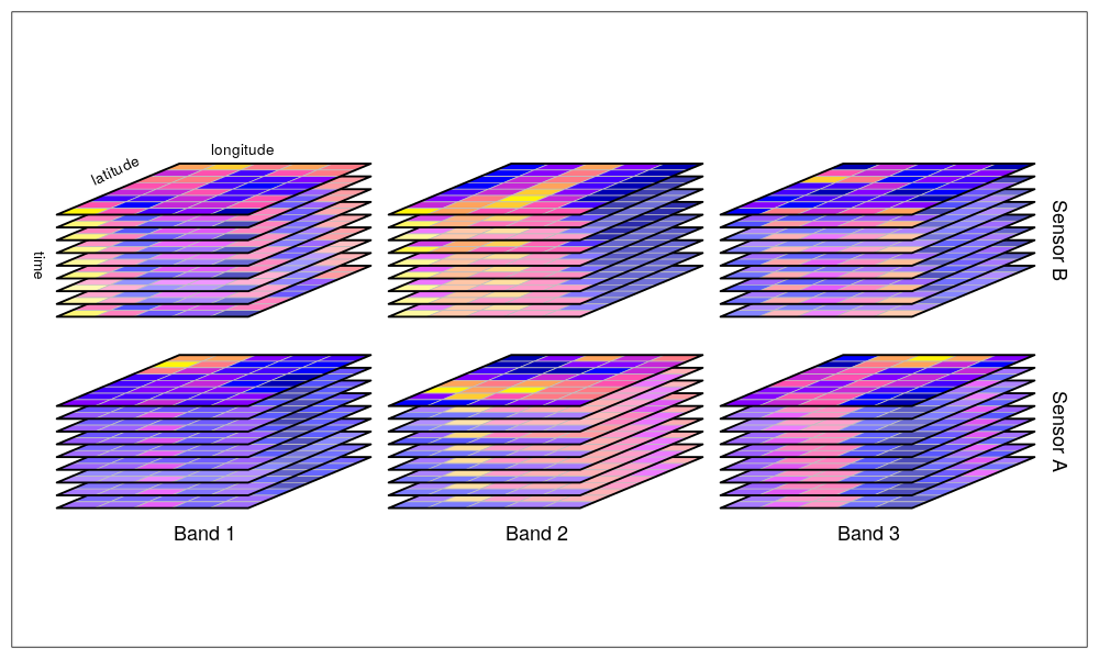
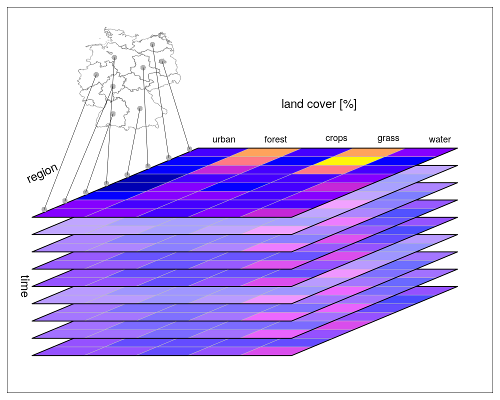
It would be great to create a figure similar to the one below from https://r-spatial.github.io/stars/, but using tmap.
@mtennekes do you have any idea if this can be done programmatically?

I came across another potentially interesting dataset, the world innovation index. It is an index based 7 pillars, from which the first 5 are related to input (what does the government in order to increase innovation), and the latter 2 to output (what innovation does the society create).

There is a yearly time series from 2013 to 2019:

Also interesting is the difference between 2019 and 2013:

As you can see, there are quite some countries without data. Let me know if this could be useful for the book. If so, I will clean up the script and make it reproducible.

@mtennekes two open questions:

1. Shapes for symbols: they work for both categorical and sequential data. However, should they work for sequential data?
2. Shapes (lty) for lines: right now it is only possible to set one line type for all of the data. Would it be possible to allow to provide a categorical variable here?

library(tmap)
data("rivers", package = "tmap")
data("metro", package = "tmap")
set.seed(222)
metro2 = metro[sample(1:nrow(metro), 30), ]
set.seed(231)
metro2$group = as.character(sample(1:3, size = nrow(metro2), replace = TRUE))

# 1 -----------------------------------------------------------------------
# works
tm_shape(metro2) +
  tm_symbols(shape = "group")
#> Linking to GEOS 3.8.1, GDAL 3.0.4, PROJ 6.3.2

# also works - but should it?
tm_shape(metro2) +
  tm_symbols(shape = "pop1950")
#> Warning: Not enough symbol shapes available. Shapes will be re-used.

# 2 -----------------------------------------------------------------------
# works
tm_shape(rivers) + 
  tm_lines(lty = 2)

# does not work
tm_shape(rivers) + 
  tm_lines(lty = "type")
#> Error in grid.Call.graphics(C_lines, x$x, x$y, index, x$arrow): invalid hex digit in 'color' or 'lty'

^{Created on 2020-11-10 by the reprex package (v0.3.0)}

It would be great to create a figure similar to the one below from https://r-spatial.github.io/stars/, but using tmap.
@mtennekes do you have any idea if this can be done programmatically?

Hi! The following reprex should present the datasets.

# load packages
library(sf)
#> Linking to GEOS 3.8.0, GDAL 3.0.4, PROJ 6.3.1
library(pct)
library(od)
library(stats19)
library(spdep)
library(igraph)
library(tmap)

First, I download MSOA data for the West-Yorkshire region (polygonal data)

west_yorkshire_msoa <- get_pct_zones("west-yorkshire", geography = "msoa") %>% 
  st_transform(27700)

The MSOA areas are defined here. Then, I download OD data for the West-Yorkshire region

west_yorkshire_od <- get_od("west-yorkshire", type = "to")

and transform them, adding a LINESTRING between the centroids of each pair of MSOAs

west_yorkshire_od <- od_to_sf(west_yorkshire_od, west_yorkshire_msoa)
#> 0 origins with no match in zone ids
#> 42084 destinations with no match in zone ids
#>  points not in od data removed.

This is the result

west_yorkshire_od[1:5, c(15, 16, 3)]
#> Simple feature collection with 5 features and 3 fields
#> geometry type:  LINESTRING
#> dimension:      XY
#> bbox:           xmin: 404584 ymin: 444696.1 xmax: 416264.8 ymax: 448081.3
#> projected CRS:  OSGB 1936 / British National Grid
#>      geo_name1    geo_name2 all                       geometry
#> 1 Bradford 001 Bradford 001 168 LINESTRING (409188.6 447966...
#> 2 Bradford 001 Bradford 002 332 LINESTRING (409188.6 447966...
#> 3 Bradford 001 Bradford 003  16 LINESTRING (409188.6 447966...
#> 4 Bradford 001 Bradford 004  86 LINESTRING (409188.6 447966...
#> 5 Bradford 001 Bradford 005  12 LINESTRING (409188.6 447966...

Each row should represent the number of commuters that, every day, go from one MSOA to the same or another MSOA. The data come from 2011 census. For example, in the following map I represent the OD line that "arrive" at "E02006875", which is the code for the MSOA at Leeds city center. Clearly, most of the commuters live nearby their workplace.

tm_shape(west_yorkshire_msoa) + 
  tm_borders() + 
tm_shape(west_yorkshire_od[west_yorkshire_od$geo_code2 == "E02006875", ]) + 
  tm_lines(
    col = "all", 
    style = "headtails", 
    palette = "-magma", 
    style.args = list(thr = 0.5), 
    lwd = 1.33
  )

Now I download car crashes data for England

england_crashes_2019 <- get_stats19(2019, output_format = "sf", silent = TRUE)

and filter the events located in the west-yorkshire region. The polygonal boundary for the west-yorkshire region is created by st-unioning the MSOA zones (after rouding all coordinates to the nearest 10s of meter).

st_precision(west_yorkshire_msoa) <- units::set_units(10, "m")
idx <- st_contains(st_union(west_yorkshire_msoa), england_crashes_2019)
west_yorkshire_crashes_2019 <- england_crashes_2019[unlist(idx), ]

I can now count the occurrences in each MSOA

west_yorkshire_msoa$number_of_car_crashes_2019 <- lengths(
  st_contains(west_yorkshire_msoa, west_yorkshire_crashes_2019)
)

and plot the result. The first map represents the location of all car crashes that occurred in the West-Yorkshire during 2019, while the second map is a choropleth map of car crashes counts in each MSOA zone.

p1 <- tm_shape(west_yorkshire_msoa) + 
  tm_borders() + 
tm_shape(west_yorkshire_crashes_2019) + 
  tm_dots(size = 0.005)
p2 <- tm_shape(west_yorkshire_msoa) + 
  tm_polygons(
    col = "number_of_car_crashes_2019", 
    style = "headtails", 
    title = ""
  )
tmap_arrange(p1, p2)

I don't live in Yorkshire but I think that the second map clearly highlights the cities of Leeds, Bradford and Wakefield. The same procedure can be repeated for 2011-2018, creating a simple animation. First I need to download and filter car crashes data for 2011-2019. Warning: the following command may take some time to run

england_crashes_2011_2019 <- get_stats19(2011:2019, output_format = "sf")
idx <- st_contains(st_union(west_yorkshire_msoa), england_crashes_2011_2019)
west_yorkshire_crashes_2011_2019 <- england_crashes_2011_2019[unlist(idx), ]

Then, I need to estimate the number of car crashes per MSOA per year:

west_yorkshire_msoa_spacetime <- do.call("rbind", lapply(
  X = 2011:2019, # the chosen years
  FUN = function(year) {
    id_year <- format(west_yorkshire_crashes_2011_2019$date, "%Y") == as.character(year)
    subset_crashes <- west_yorkshire_crashes_2011_2019[id_year, ]
    st_sf(
      data.frame(
        number_car_crashes = lengths(st_contains(west_yorkshire_msoa, subset_crashes)), 
        year = year
      ), 
      geometry = st_geometry(west_yorkshire_msoa)
    )
  }
))

And create the animation

tmap_animation(
  tm_shape(west_yorkshire_msoa_spacetime) + 
    tm_polygons(col = "number_car_crashes", style = "headtails") + 
    tm_facets(along = "year"), 
  filename = "tests_tmap.gif", 
  delay = 100
)

The car crashes focus more or less always in the same areas (for obvious reasons) and they seem to be more and more focused around the big cities.

Now I want to estimate a traffic measure for each MSOA zone (to be used as an offset in a car crashes model, offtopic here). The problem with raw OD data is that they ignore the fact that people may travel to their workplace through several MSOAs (@Robinlovelace please correct me here). So I estimate a traffic measure using the following approximation. First I build a neighbours list starting from the MSOA regions:

west_yorkshire_queen_nb <- poly2nb(west_yorkshire_msoa, snap = 10)

I think this is more or less equivalent to queen_nb_west_yorkshire <- st_relate(msoa_west_yorkshire, pattern = "F***T****") since we set st_precision(msoa_west_yorkshire) <- units::set_units(10, "m"). I'm not sure how to visualise nb objects with tmap (but I think it could be a nice extension, if absent), so I will use base R + spdep for the moment:

par(mar = rep(0, 4))
plot(st_geometry(west_yorkshire_msoa))
plot(west_yorkshire_queen_nb, st_centroid(st_geometry(west_yorkshire_msoa)), add = TRUE)

The lines connect the centroid of each MSOA with the centroids of all neighbouring MSOA. This structure is useful since it uniquely determines the adjacency matrix of a graph that can be used to estimate the (approximate) shortest path between two MSOA (i.e. the Origin and the Destination).

west_yorkshire_graph <- graph_from_adjacency_matrix(nb2mat(west_yorkshire_queen_nb, style = "B"))
west_yorkshire_graph
#> IGRAPH b1a7661 D--- 299 1716 -- 
#> + edges from b1a7661:
#>  [1]  1->  2  1->  3  1->  4  1->  5  1->  6  1-> 10  2->  1  3->  1  3->  5
#> [10]  3->150  3->151  4->  1  4->  6  4->  7  4-> 14  5->  1  5->  3  5->  6
#> [19]  5-> 10  5->151  5->155  6->  1  6->  4  6->  5  6->  7  6->  8  6-> 10
#> [28]  6-> 15  7->  4  7->  6  7->  8  7->  9  7-> 14  8->  6  8->  7  8->  9
#> [37]  8-> 11  8-> 15  8-> 31  9->  7  9->  8  9-> 11  9-> 12  9-> 14 10->  1
#> [46] 10->  5 10->  6 10-> 13 10-> 15 10-> 18 10->155 11->  8 11->  9 11-> 12
#> [55] 11-> 14 11-> 23 11-> 31 12->  9 12-> 11 12-> 14 13-> 10 13-> 16 13-> 17
#> [64] 13-> 18 13->155 14->  4 14->  7 14->  9 14-> 11 14-> 12 14-> 23 15->  6
#> [73] 15->  8 15-> 10 15-> 18 15-> 22 15-> 31 16-> 13 16-> 17 16-> 18 16-> 20
#> + ... omitted several edges

That graph has 299 vertices (the number of MSOA in West Yorkshire) and 1716 edges (the lines visualised in the previous plot). Now I'm going to "decorate" that graph by assigning to each edge a weight that is equal to the geographical distance between the centroids that define the edge. First I need the edgelist:

west_yorkshire_edgelist <- as_edgelist(west_yorkshire_graph) 

and then I can estimate the distances

E(west_yorkshire_graph)$weight <- units::drop_units(st_distance(
  x = st_centroid(st_geometry(west_yorkshire_msoa))[west_yorkshire_edgelist[, 1]], 
  y = st_centroid(st_geometry(west_yorkshire_msoa))[west_yorkshire_edgelist[, 2]], 
  by_element = TRUE
)) 

I can also assign a name to each vertex equal to the corresponding MSOA code:

V(west_yorkshire_graph)$name <- west_yorkshire_msoa[["geo_code"]]

This is the result, with an analogous interpretation as before

west_yorkshire_graph
#> IGRAPH b1a7661 DNW- 299 1716 -- 
#> + attr: name (v/c), weight (e/n)
#> + edges from b1a7661 (vertex names):
#>  [1] E02002183->E02002184 E02002183->E02002185 E02002183->E02002186
#>  [4] E02002183->E02002187 E02002183->E02002188 E02002183->E02002192
#>  [7] E02002184->E02002183 E02002185->E02002183 E02002185->E02002187
#> [10] E02002185->E02002332 E02002185->E02002333 E02002186->E02002183
#> [13] E02002186->E02002188 E02002186->E02002189 E02002186->E02002196
#> [16] E02002187->E02002183 E02002187->E02002185 E02002187->E02002188
#> [19] E02002187->E02002192 E02002187->E02002333 E02002187->E02002337
#> [22] E02002188->E02002183 E02002188->E02002186 E02002188->E02002187
#> + ... omitted several edges

Now I'm going to loop over all OD lines, calculate the shortest path between the Origin and Destination MSOA, and assign to each MSOA in the shortest path a traffic measure that is proportional to the number of people that commute using that OD line. I know that it sounds a little confusing but I can write it better if you like the idea:

west_yorkshire_msoa$traffic <- 0 # initialize the traffic column

pb <- txtProgressBar(min = 1, max = nrow(west_yorkshire_od), style = 3)
for (i in seq_len(nrow(west_yorkshire_od))) {
  origin <- west_yorkshire_od[["geo_code1"]][i]
  destination <- west_yorkshire_od[["geo_code2"]][i]
  
  if (origin == destination) { # this should be an "intrazonal" 
    idx <- which(west_yorkshire_msoa$geo_code == origin)
    west_yorkshire_msoa$traffic[idx] <- west_yorkshire_msoa$traffic[idx] + west_yorkshire_od[["all"]][i]
    # west_yorkshire_msoa$traffic[idx] is the previous value while
    # west_yorkshire_od[["all"]][i] is the "new" traffic value
    next()
  }
  
  # Estimate shortest path
  idx_geo_code <- as_ids(shortest_paths(west_yorkshire_graph, from = origin, to = destination)$vpath[[1]])
  idx <- which(west_yorkshire_msoa$geo_code %in% idx_geo_code)
  west_yorkshire_msoa$traffic[idx] <- west_yorkshire_msoa$traffic[idx] + (west_yorkshire_od[["all"]][i] / length(idx))
  # west_yorkshire_msoa$traffic[idx] are the previous values while
  # west_yorkshire_od[["all"]][i] is the new traffic count (divided by the
  # number of MSOAs in the shortest path)
  
  setTxtProgressBar(pb, i)
}

For example, if i = 53778, then

west_yorkshire_od[53778, 1:3]
#> Simple feature collection with 1 feature and 3 fields
#> geometry type:  LINESTRING
#> dimension:      XY
#> bbox:           xmin: 415279.3 ymin: 418009.9 xmax: 430001.7 ymax: 433379.7
#> projected CRS:  OSGB 1936 / British National Grid
#>       geo_code1 geo_code2 all                       geometry
#> 53778 E02006875 E02002299  18 LINESTRING (430001.7 433379...

i.e. the number of daily commuters is equal to 18, while the shortest path between E02006875 and E02002299 is given by

shortest_path_example <- shortest_paths(west_yorkshire_graph, "E02006875", "E02002299", output = "both")
shortest_path_example
#> $vpath
#> $vpath[[1]]
#> + 12/299 vertices, named, from b1a7661:
#>  [1] E02006875 E02002411 E02002419 E02002422 E02002433 E02002435 E02002276
#>  [8] E02002281 E02002285 E02002302 E02002307 E02002299
#> 
#> 
#> $epath
#> $epath[[1]]
#> + 11/1716 edges from b1a7661 (vertex names):
#>  [1] E02006875->E02002411 E02002411->E02002419 E02002419->E02002422
#>  [4] E02002422->E02002433 E02002433->E02002435 E02002435->E02002276
#>  [7] E02002276->E02002281 E02002281->E02002285 E02002285->E02002302
#> [10] E02002302->E02002307 E02002307->E02002299
#> 
#> 
#> $predecessors
#> NULL
#> 
#> $inbound_edges
#> NULL

It would be nice to represent the "shortest path" like the previous map (and check the results) but I'm not sure how to do that right now.

Now, we can compare the traffic estimates with the car crashes counts:

p1 <- tm_shape(west_yorkshire_msoa) + 
  tm_polygons(
    col = "number_of_car_crashes_2019", 
    style = "headtails", 
    title = ""
  )
p2 <- tm_shape(west_yorkshire_msoa) + 
  tm_polygons(
    col = "traffic", 
    style = "headtails", 
    title = ""
  )
tmap_arrange(p1, p2)

The scales are quite different (obviously), but they highlight the same areas (which is not incredible, but still...)

I think that the examples presented here are nice since they are related to a "real-world application" with open data (with some licence limitation maybe, I don't know). I think that the visualisation component should be stressed much more (and the maps related to neighborhood matrices should be implemented with tmap). This example is probably too difficult for a book not related to road safety or models for car crashes, but if you like it I think we can organize something!

^{Created on 2020-10-10 by the reprex package (v0.3.0)}

devtools::session_info()
#> - Session info ---------------------------------------------------------------
#>  setting  value                       
#>  version  R version 3.6.3 (2020-02-29)
#>  os       Windows 10 x64              
#>  system   x86_64, mingw32             
#>  ui       RTerm                       
#>  language (EN)                        
#>  collate  Italian_Italy.1252          
#>  ctype    Italian_Italy.1252          
#>  tz       Europe/Berlin               
#>  date     2020-10-10                  
#> 
#> - Packages -------------------------------------------------------------------
#>  package      * version    date       lib source                              
#>  abind          1.4-5      2016-07-21 [1] CRAN (R 3.6.0)                      
#>  assertthat     0.2.1      2019-03-21 [1] CRAN (R 3.6.0)                      
#>  backports      1.1.10     2020-09-15 [1] CRAN (R 3.6.3)                      
#>  base64enc      0.1-3      2015-07-28 [1] CRAN (R 3.6.0)                      
#>  boot           1.3-25     2020-04-26 [1] CRAN (R 3.6.3)                      
#>  callr          3.4.4      2020-09-07 [1] CRAN (R 3.6.3)                      
#>  class          7.3-17     2020-04-26 [1] CRAN (R 3.6.3)                      
#>  classInt       0.4-3      2020-04-07 [1] CRAN (R 3.6.3)                      
#>  cli            2.0.2      2020-02-28 [1] CRAN (R 3.6.3)                      
#>  coda           0.19-3     2019-07-05 [1] CRAN (R 3.6.1)                      
#>  codetools      0.2-16     2018-12-24 [2] CRAN (R 3.6.3)                      
#>  crayon         1.3.4      2017-09-16 [1] CRAN (R 3.6.0)                      
#>  crosstalk      1.1.0.1    2020-03-13 [1] CRAN (R 3.6.3)                      
#>  curl           4.3        2019-12-02 [1] CRAN (R 3.6.1)                      
#>  DBI            1.1.0      2019-12-15 [1] CRAN (R 3.6.3)                      
#>  deldir         0.1-29     2020-09-13 [1] CRAN (R 3.6.3)                      
#>  desc           1.2.0      2018-05-01 [1] CRAN (R 3.6.0)                      
#>  devtools       2.3.2      2020-09-18 [1] CRAN (R 3.6.3)                      
#>  dichromat      2.0-0      2013-01-24 [1] CRAN (R 3.6.0)                      
#>  digest         0.6.25     2020-02-23 [1] CRAN (R 3.6.3)                      
#>  dplyr          1.0.2      2020-08-18 [1] CRAN (R 3.6.3)                      
#>  e1071          1.7-3      2019-11-26 [1] CRAN (R 3.6.1)                      
#>  ellipsis       0.3.1      2020-05-15 [1] CRAN (R 3.6.3)                      
#>  evaluate       0.14       2019-05-28 [1] CRAN (R 3.6.0)                      
#>  expm           0.999-5    2020-07-20 [1] CRAN (R 3.6.3)                      
#>  fansi          0.4.1      2020-01-08 [1] CRAN (R 3.6.2)                      
#>  fs             1.5.0      2020-07-31 [1] CRAN (R 3.6.3)                      
#>  gdata          2.18.0     2017-06-06 [1] CRAN (R 3.6.0)                      
#>  generics       0.0.2      2018-11-29 [1] CRAN (R 3.6.0)                      
#>  gifski         0.8.6      2018-09-28 [1] CRAN (R 3.6.0)                      
#>  glue           1.4.2      2020-08-27 [1] CRAN (R 3.6.3)                      
#>  gmodels        2.18.1     2018-06-25 [1] CRAN (R 3.6.1)                      
#>  gtools         3.8.2      2020-03-31 [1] CRAN (R 3.6.3)                      
#>  highr          0.8        2019-03-20 [1] CRAN (R 3.6.0)                      
#>  hms            0.5.3      2020-01-08 [1] CRAN (R 3.6.2)                      
#>  htmltools      0.5.0      2020-06-16 [1] CRAN (R 3.6.3)                      
#>  htmlwidgets    1.5.1      2019-10-08 [1] CRAN (R 3.6.1)                      
#>  httr           1.4.2      2020-07-20 [1] CRAN (R 3.6.3)                      
#>  igraph       * 1.2.5      2020-03-19 [1] CRAN (R 3.6.3)                      
#>  KernSmooth     2.23-17    2020-04-26 [1] CRAN (R 3.6.3)                      
#>  knitr          1.30       2020-09-22 [1] CRAN (R 3.6.3)                      
#>  lattice        0.20-41    2020-04-02 [1] CRAN (R 3.6.3)                      
#>  leafem         0.1.3      2020-07-26 [1] CRAN (R 3.6.3)                      
#>  leaflet        2.0.3      2019-11-16 [1] CRAN (R 3.6.3)                      
#>  leafsync       0.1.0      2019-03-05 [1] CRAN (R 3.6.1)                      
#>  LearnBayes     2.15.1     2018-03-18 [1] CRAN (R 3.6.0)                      
#>  lifecycle      0.2.0      2020-03-06 [1] CRAN (R 3.6.2)                      
#>  lwgeom         0.2-5      2020-06-12 [1] CRAN (R 3.6.3)                      
#>  magrittr       1.5        2014-11-22 [1] CRAN (R 3.6.3)                      
#>  MASS           7.3-53     2020-09-09 [1] CRAN (R 3.6.3)                      
#>  Matrix         1.2-18     2019-11-27 [2] CRAN (R 3.6.3)                      
#>  memoise        1.1.0      2017-04-21 [1] CRAN (R 3.6.0)                      
#>  mime           0.9        2020-02-04 [1] CRAN (R 3.6.2)                      
#>  nlme           3.1-149    2020-08-23 [1] CRAN (R 3.6.3)                      
#>  od           * 0.0.1      2020-09-09 [1] CRAN (R 3.6.3)                      
#>  pct          * 0.5.0      2020-08-27 [1] CRAN (R 3.6.3)                      
#>  pillar         1.4.6      2020-07-10 [1] CRAN (R 3.6.3)                      
#>  pkgbuild       1.1.0      2020-07-13 [1] CRAN (R 3.6.3)                      
#>  pkgconfig      2.0.3      2019-09-22 [1] CRAN (R 3.6.1)                      
#>  pkgload        1.1.0      2020-05-29 [1] CRAN (R 3.6.3)                      
#>  png            0.1-7      2013-12-03 [1] CRAN (R 3.6.0)                      
#>  prettyunits    1.1.1      2020-01-24 [1] CRAN (R 3.6.2)                      
#>  processx       3.4.4      2020-09-03 [1] CRAN (R 3.6.3)                      
#>  ps             1.3.4      2020-08-11 [1] CRAN (R 3.6.3)                      
#>  purrr          0.3.4      2020-04-17 [1] CRAN (R 3.6.3)                      
#>  R6             2.4.1      2019-11-12 [1] CRAN (R 3.6.1)                      
#>  raster         3.3-13     2020-07-17 [1] CRAN (R 3.6.3)                      
#>  RColorBrewer   1.1-2      2014-12-07 [1] CRAN (R 3.6.0)                      
#>  Rcpp           1.0.5      2020-07-06 [1] CRAN (R 3.6.3)                      
#>  readr          1.3.1      2018-12-21 [1] CRAN (R 3.6.0)                      
#>  remotes        2.2.0      2020-07-21 [1] CRAN (R 3.6.3)                      
#>  rlang          0.4.7      2020-07-09 [1] CRAN (R 3.6.3)                      
#>  rmarkdown      2.3        2020-06-18 [1] CRAN (R 3.6.3)                      
#>  rprojroot      1.3-2      2018-01-03 [1] CRAN (R 3.6.0)                      
#>  sessioninfo    1.1.1      2018-11-05 [1] CRAN (R 3.6.0)                      
#>  sf           * 0.9-6      2020-09-13 [1] CRAN (R 3.6.3)                      
#>  sfheaders      0.2.2      2020-05-13 [1] CRAN (R 3.6.3)                      
#>  sp           * 1.4-2      2020-05-20 [1] CRAN (R 3.6.3)                      
#>  spData       * 0.3.8      2020-07-03 [1] CRAN (R 3.6.3)                      
#>  spDataLarge    0.3.1      2019-06-30 [1] Github (Nowosad/spDataLarge@012fe53)
#>  spdep        * 1.1-5      2020-06-29 [1] CRAN (R 3.6.3)                      
#>  stars          0.4-4      2020-08-19 [1] Github (r-spatial/stars@b7b54c8)    
#>  stats19      * 1.3.0      2020-09-30 [1] local                               
#>  stringi        1.4.6      2020-02-17 [1] CRAN (R 3.6.2)                      
#>  stringr        1.4.0      2019-02-10 [1] CRAN (R 3.6.0)                      
#>  testthat       2.3.2      2020-03-02 [1] CRAN (R 3.6.3)                      
#>  tibble         3.0.3.9000 2020-07-12 [1] Github (tidyverse/tibble@a57ad4a)   
#>  tidyselect     1.1.0      2020-05-11 [1] CRAN (R 3.6.3)                      
#>  tmap         * 3.2        2020-09-15 [1] CRAN (R 3.6.3)                      
#>  tmaptools      3.1        2020-07-12 [1] Github (mtennekes/tmaptools@947f3bd)
#>  units          0.6-7      2020-06-13 [1] CRAN (R 3.6.3)                      
#>  usethis        1.6.3      2020-09-17 [1] CRAN (R 3.6.3)                      
#>  vctrs          0.3.4      2020-08-29 [1] CRAN (R 3.6.3)                      
#>  viridisLite    0.3.0      2018-02-01 [1] CRAN (R 3.6.0)                      
#>  withr          2.3.0      2020-09-22 [1] CRAN (R 3.6.3)                      
#>  xfun           0.17       2020-09-09 [1] CRAN (R 3.6.3)                      
#>  XML            3.99-0.3   2020-01-20 [1] CRAN (R 3.6.2)                      
#>  xml2           1.3.2      2020-04-23 [1] CRAN (R 3.6.3)                      
#>  yaml           2.2.1      2020-02-01 [1] CRAN (R 3.6.2)                      
#> 
#> [1] C:/Users/Utente/Documents/R/win-library/3.6
#> [2] C:/Program Files/R/R-3.6.3/library

@mtennekes could you tell me (or point me to the code) how tm_text() relates to other layer types. I assume it just uses coordinates of points, and centroids (??) of lines and polygons?

• https://doi.org/10.18637/jss.v084.i06
• https://cran.r-project.org/package=tmap/vignettes/tmap-getstarted.html
• https://cran.r-project.org/package=tmap/vignettes/tmap-changes.html
• http://stackoverflow.com/questions/tagged/tmap
• https://mtennekes.github.io/downloads/presentations/tmap_user2015.pdf
• https://github.com/mtennekes/tmap-workshop
• http://www.computerworld.com/article/2921176/business-intelligence/great-r-packages-for-data-import-wrangling-visualization.html
• http://www.computerworld.com/article/3175623/data-analytics/mapping-in-r-just-got-a-whole-lot-easier.html
• https://sesync-ci.github.io/maps-in-R-lesson/
• http://geocompr.robinlovelace.net/adv-map.html
• https://mtennekes.github.io/downloads/presentations/tmap_user2017.pdf
• https://gotellilab.github.io/Bio381/StudentPresentations/SpatialDataTutorial.html
• https://mtennekes.github.io/downloads/presentations/tmap_opengeo_muenster.pdf
• https://www.youtube.com/watch?v=wgFVmzSbaQc#t=3m20s
• https://geocompr.github.io/tags/tmap/

@mtennekes can you help me here. I have seen the examples (they look great BTW), but I have also tried to create my own cases and failed. You can see two of them below.

library(tmap)
library(grid)
library(ggplotify)
library(ggplot2)
data("metro", package = "tmap")

set.seed(222)
metro2 = metro[sample(1:nrow(metro), 30), ]
set.seed(231)
metro2$group = as.character(sample(1:3, size = nrow(metro2), replace = TRUE))

p1 = as.grob(~barplot(1:10))
p2 = as.grob(expression(plot(rnorm(10))))
p3 = as.grob(function() plot(sin))
p4 = ggplotGrob(ggplot(data.frame(x = 1:10, y = 1:10), aes(x, y)) + geom_point())

# what is wrong here?
tm_shape(metro2) +
  tm_symbols(shape = "group",
             shapes = list(p4, p4, p4)) 
#> Linking to GEOS 3.8.1, GDAL 3.0.4, PROJ 6.3.2

# is anything like this is even possible?
tm_shape(metro2) +
  tm_symbols(shape = "group",
             shapes = list(p1, p2, p3)) 

^{Created on 2020-11-09 by the reprex package (v0.3.0)}

I have an idea for a figure explaining visual variables. It could be a grid with three columns and four rows:

• Columns - represent data types (1. symbols, 2. lines, 3. polygons)
• Rows - represent visual variables (1. categorical colors, 2. sequential colors, 3. shapes, 4. sizes)

Each example could be directly taken from a tmap plots' legends. For more details - visit the Visual Variables section in chapter 5. What do you think about it, @mtennekes ?

Pros:

1. People could see (and manipulate) the actual code output
2. Interactive maps are nice.

Cons:

1. Interactive maps require disabling caching and kniting all chapters together (rstudio/bookdown#15) - b6db046
2. Interactive maps have some tiny issues in bookdown, e.g.
   

When it is fixed, then some chunks should be re-enabled - 79b8551.

At least three different scales:

• Global/continental
• Regional/country level
• Local

Each level should have complete set of possible spatial object types with interesting attributes:

• Points
• Lines
• Polygons
• Categorical raster(s)
• Continuous raster(s)

At least one of the scales should also have some temporal variables to showcase tmap's animation capabilities.

I've updated the outline, see https://github.com/r-tmap/tmap-book/blob/master/meta/book-outline.Rmd

One difference with what we discussed yesterday, is that I've placed the chapter about other map types (cartogram, geogrid) as 6th. Why? Because it is a natural extension/use of the map layers, and belongs to the basic 'how to map data' part. So therefore also before layout and small multiples.

We can continue the discussion about the outline in this issue if needed.

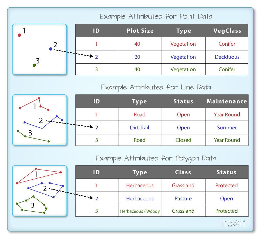
It would be great to reproduce the blow figure from https://www.earthdatascience.org/courses/earth-analytics/spatial-data-r/intro-vector-data-r/ using R code entirely.

The is a code chunk vector-data-model from https://github.com/r-tmap/tmap-book/blob/master/02-geodata.Rmd, which can be used as a starting point.