공용 서버에서 특정 계정으로 git commit 하기

• For only a single command
  • 공용 서버에서 사용하는 프로젝트에서 config 설정할 수 없는 경우 일회성 명령 사용

git -c user.name="seula.k" -c user.email="[email protected] commit -m "commit message"

• For single repository
  • 프로젝트마다 다른 이름과 이메일 주소를 사용하고 싶은 경우

git config user.name "tmfdk333"
git config user.email "[email protected]"

• For every repository on your computer
  • 시스템 전체에서 사용자 설정을 할 경우

git config --global user.name "tmfdk333"
git config --global user.email "[email protected]"

• 설정 확인
  • Git은 같은 키를 여러 파일(/etc/config, ~/.gitconfig)에서 읽을 경우, 나중 값을 사용함

git config --list

• Reference
  • 5. 시작하기 - Git 최초 설정
  • Setting your username in Git
  • Override configured user for a single git commit

Twitter Sentiment Analysis With Neural Networks

DECEMBER 20, 2016

Machine Learning, AI, and other related fields have recently been surrounded by a lot of hype. Although I'm not necessarily extremely drawn to these fields this winter quarter ended up being a perfect opportunity to at least dip my feet into them. I took two classes "Data & Knowledge Bases" and "Computer Networking" which ended up being perfect platforms to do some ML studies.

최근 기계학습, AI 등 관련 분야가 대대적으로 유행되고 있다. 나는 이 분야에 극단적으로 끌리는 것은 아니었지만, 이번 겨울은 이 분야에 발을 담그는 완벽한 기회가 되었다. 나는 "Data & Knowledge Bases"와 "Computer Networking" 두 개의 수업을 들었는데, 이 수업은 결국 몇몇 ML 연구를 위한 완벽한 기반이 되었다.

I ventured into the world of ML with two projects that aimed to use Neural Networks to solve two different problems: "Twitter Sentiment Analysis" (presented on this post) and "Spam Analysis within SoundCloud" (presented on an upcoming post).

나는 Neural Networks를 사용한 서로 다른 문제인 Twitter Sentiment Analysis(현재 포스트)와 Spam Analysis within SoundCloud(다음 포스트) 두 가지 프로젝트를 가지고 ML의 세계로 뛰어들었다.

1. The "Motivation": Twitter Sentiment Analysis

While the main motivation behind this project was to learn, understand, and ultimately hand code a Neural Networks, we decided to frame all of our efforts to do Twitter sentiment analysis. In other words, we were attempting to use our NN to distinguish whether any given tweet is of positive (happy, funny, etc.) or negative (angry, sad, etc.) sentiment.

이 프로젝트의 주된 목적은 신경망을 배우고 이해하고 궁극적으로 코드를 작성하는 것이었지만, Twitter 감정 분석에 더 노력하기로 결정했다. 즉, NN을 사용하여 주어진 트윗이 긍정적(행복, 재미 등)인지, 부정적인(분노, 슬픔 등)인지 등을 구별하려고 했다.

2. The Dataset

Our dataset consisted of a huge list of roughly 1.5M tweets that had been labeled as good or bad sentiment. The dataset contained tweets labeled by the University of Michigan and Niek Sanders. Our dataset can be found here. Notice than when training and testing we simply sampled random subsets of this dataset.

데이터셋은 좋음과 나쁨이라는 감정 꼬리표가 붙은 약 1.5만 트윗의 큰 목록으로 구성되었다. 데이터셋에는 University of Michigan의 Niek Sanders가 라벨을 붙인 트윗이 들어있었다. 데이터셋은 여기에서 찾을 수 있다. 우리가 training과 testing을 할 때 이 데이터셋의 하위 집합을 간단한 방법으로 랜덤 샘플링하여 사용했단 것을 주의해야 한다.

3. The Intuition behind Neural Networks

The truth is that to best understand the inner workings of Neural Networks I would suggest checking out Nielsen's or Trask's work, because they do a fantastic job at presenting the subject. Alternatively, you can take a look at our work were we condensed all of these ideas there. However, I wanted to attempt to convey a simple understanding of how these NNs work.

사실, NN의 내부 동작을 가장 잘 이해하기 위해 Nielsen과 Trask의 작업을 확인해 볼 것을 제안하고 싶다. 그들은 NN의 내부 동작에 대한 주제를 표현하는 데 환상적인 글을 작성했기 때문이다. 그 대신 당신은 Nielsen과 Trask의 아이디어들을 고려한 우리의 작업을 볼 수 있다. 나는 NN의 동작 방법에 대한 간단한 이해를 전달하고 싶었다.

An NN is essentially trying to emulate a brain. The NN will have a set of nodes (neurons) connected between each other (these connections are equivalent to synapses). The most basic NNs, called Feed-Forward NNs, have an input layer (of nodes), an output layer, and in the middle a variable number of "hidden layers". Each layer consists of a number of nodes that are fully connected to both the layers before and after them. These NNs have two possible operations: Forward Propagation and Backpropagation.

NN는 근본적으로 뇌를 모방하려고 한다. NN에는 노드의 집합(뉴런들)이 서로 연결되어 있다(이 연결은 시냅스와 같다). Feed-Forward NNs라고 불리는 가장 기본적인 NN은 input layer(노드의 input layer), output layer, 그리고 중간에는 variable number의 hidden layers를 가지고 있다. 각 layer는 자신의 이전/이후 두 계층 모두에 완전히 연결(fully connected)되는 다수의 노드로 구성된다. 이러한 NN에는 Forward Propagation과 Backpropagation 두 가지 작업이 있다.

• Neural Network Structure

3-1) Forward Propagation

Forward Propagation is a method used to calculate the value of a node
given all the previous nodes connected to it. If we focus on the picture above, The value of the 2a node is dictated by the values of 1a, 1b, 1c. Now notice that each connection will have its own weight (this is equivalent to how close the neurons are in a brain; the closer, the easier it is for a neuron to activate the other. the further, the harder it will be.)

Forward Propagation은 연결된 이전 모든 노드들의 값으로 현재 노드의 값을 계산하는 방법이다. 위의 그림을 보면2a 노드의 값은 1a, 1b, 1c의 값에 의해 결정된다. 이제 각각의 연결이 자체 weight를 갖게 되는 것을 알 수 있다. (이것은 뇌에서 뉴런들이 얼마나 가까이에 있는지 알 수 있다. 가까울수록 뉴런이 다른 뉴런을 활성화시키기 쉬울 것이고, 멀수록 뉴런이 다른 뉴런을 활성화시키기 어려울 것이다.)

Furthermore within the node 2a there is an activation function which essentially normalizes it's own value to something between 0 and 1 (although different activation functions can be used for different purposes.)

또한 노드 2a에는 근본적으로 자신의 값을 0과 1 사이의 어떤 것으로 normalize하는 activation function(활성화 함수)이 있다. (비록 다른 activation function을 다른 목적으로 사용할 수 있다.)

So the final result is that value of 2a = activation(w1(value of 1a) + w2(value of 2a) + w3(value of 1c)).

따라서 결론적으로 2a의 값 = activation_function(w1(1a의 값) + w2(1b의 값) + w3(1c의 값)) 이다.

If one keeps doing this for all nodes, one can calculate the output of any given input. This is needed for both the training and testing phase, except that in the training phase a forward propagation is immediately followed by a backpropagation.

모든 노드에 대해 계속 이 작업을 수행하면 주어진 input의 ouput을 계산할 수 있다. 이는 training/testing 단계 모두에서 필요하다. 단, training 단계에서는 forward propagation 다음에 즉시 backpropagation이 뒤따르는 점을 제외한다.

3-2) Backpropagation

Backpropagation is a method used only during the training phase. After running the forward propagation on an NN, we calculate the error obtained between our output and our expected output and we use backpropagation to fix (or diminish) that error. Backpropagation essentially allows neurons to re-adjust their weights in such a way that given a specific input, the proper output will be returned. the exact mathematics of this are a bit convoluted so I'd rather point you to our paper to further understand the maths.

Backpropagation은 training 단계에서만 사용하는 방법이다. NN에서 forward propagation을 실행한 후에 원래의 output과 예상된 output 사이에서 얻어진 오류를 계산하고, 오류를 수정(또는 감소)하기 위해 backpropagation을 사용한다. Backpropagation은 기본적으로 뉴런이 특정 input을 받으면 적절한 output이 반환되는 방식으로 weight를 다시 조정할 수 있게 한다. Backpropagation의 정확한 수학은 조금 복잡하기 때문에 수학적으로 더욱 깊이 이해하기 위해서는 아래의 논문을 참조한다.

4. Representing Tweets

As you may have already noticed our NN accepts only numbers as inputs. Thus, we needed to find a way to represent tweets as numbers without loosing too much information. We knew that doing something simple as hashing each word wouldn't work because you loose the relation and even meaning of words. For example; Imagine HATE = 1001 and LOVE = 1000; The two words are way to similar and the NN will activate equally for both. So instead, we started tinkering around and tried 3 different methods.

이미 알고 있었겠지만 NN은 숫자만 input으로 받아들인다. 따라서, 너무 많은 정보를 잃지 않고 트윗을 숫자로 나타낼 수 있는 방법을 찾아야 했다. 단어의 의미와 관계를 잃어버릴 것이기 때문에 각 단어를 해싱하는 것과 같은 간단한 작업은 효과가 없을 것이라는 것을 알고 있었다. 예를들면 HATE=1001, LOVE=1000이라고 상상해보자. 두 단어는 비슷한 방법이고, NN은 둘 다 동일하게 활성화될 것이다. 그래서 대신 우리는 3가지 다른 방법을 시도했다.

4-1) Bayesian Probabilities

Our first very naive approach was very similar to applying Naive Bayes Classifier. We calculated the probabilities that each word in the dataset was good or bad and then fed that as the input to our Neural Network.

첫 번째로 시도한 순진한 접근 방법은 Naive Bayes Classifier를 적용하는 것과 매우 유사했다. 우리는 데이터셋에서 각 단어가 좋거나 나쁘다는 확률을 계산한 다음 이 확률을 Neural Network의 input으로 제공했다.

• Bayesian Probabilities Representation

This provided results of around 63%, which were good, but not great. Furthermore, we found that it performed nearly identically to a Bayesian Classifier, which meant we were simply going a really complicated way to achieve the same results. Thus, although it was an interesting starting point, it was a rather poor tweet representation.

이것은 약 63%의 결과를 제공했는데, 이것은 좋긴 했지만 훌륭하지는 않았다. 게다가 Bayesian Classifier와 거의 동일하게 동작한다는 것을 알았다. 이 말은 결국 같은 결과를 얻기 위해서 매우 복잡한 길을 가고 있다는 것을 의미한다. 따라서 흥미로운 시작점이긴 했지만, 매우 형편없는 tweet representation이었다.

4-2) Word Embeddings

We heard lots of cool things about word embeddings and decided to try them out. Word Embeddings are a rather new method of describing words in a dictionary by mapping them into n-dimensional fields. The actual methodology varies depending on the authors (see wiki). In our case we used Keras' built in Word Embedding layers to build our own.

우리는 word embeddings에 대해 좋은 것들을 많이 듣고 그것들을 시도하기로 결정했다. Word Embeddings는 사전에서 단어를 n차원 영역에 매핑하여 설명하는 다소 새로운 방법이다. 실제 방법론은 저자에 따라 다양하다(wiki 참조). 우리의 경우, 우리의 것을 만들기 위해서 Keras' built in Word Embedding layers를 사용했다.

• Word Embeddings

Although we originally thought this was going to give us fantastic results, we actually obtained poorer accuracy than with plain and simple Bayesian Probabilities. We realized that this happened because Tweets are very unique literal constructs where people use lots of uncommon things such as mentions (@Someone), hashtags (#topic), and urls. Furthermore, typos and irregular abbreviations or lack of whitespace due to length constraints, made our word embeddings inaccurate.

이것이 환상적인 결과를 가져다 줄 것이라고 생각했지만, 평범하고 간단한 Bayesian 확률보다 더 낮은 정확도를 얻었다. 우리는 twitter에서 사림들이 멘션(@Someone), 해시태그(#topic), url 과 같은 독특한 문자를 많이 사용하는 구조이기 때문에 이런 일이 일어났다는 것을 깨달았다. 또한 오타, 불규칙한 약어, 길이 제한으로 인해 공백이 없어 word embedding이 부정확했다.

4-3) Feature Vector

After our "failure" with Word Embedding, we decided to go back to the drawing board. We asked ourselves: What makes a tweet a tweet? After long philosophical contemplation, we came up with a set of features that we believed described each tweet as best as possible. We came up with a long list of features that tried to capture as much information as possible. Of course, we knew that some of these features were not as useful as others and thus, we filtered the useful ones using Correlation-Based Feature Subset Selection in WEKA. This allowed us to select only the most descriptive (and non-redundant) features from our list.

Word Embedding의 실패 후, 처음부터 다시 시작하기로 결정했다. 무엇이 tweet을 tweet으로 만들까? 스스로 질문했다. 오랜 차분한 고민 끝에 우리는 각 tweet을 가능한 한 잘 표현한다고 생각되는 일련의 feature(특징)들을 찾아냈다. 가능한 한 많은 정보를 수집하기 위해서 많은 feature 리스트를 작성했다.
물론 이러한 특징들 중 일부가 다른 feature보다 유용하지 않다는 것을 알았고, WEKA에서 Correlation-Based Feature Subset Selection(연관성 기반 feature 하위집합 선택)을 사용하여 유용한 feature들을 필터링했다.

• Our feature list for tweet representation

This actually provided the best results, and we were actually able to reach near 70% accuracy. We considered this to be successful seeing how it would have landed us in the top 30 of the Kaggle Michigan University Twitter Sentiment Analysis Challenge.

이것은 실제로 최고의 결과를 제공했고, 우리는 거의 70%의 정확도에 도달할 수 있었다. 이것이 우리가 어떻게 Kaggle Michigan University Twitter Sentiment Analysis Challenge에서 상위 30위에 들 수 있었는지 볼 수 있는 성공적인 방법이라고 생각했다.

5. Our Results

On our experiments, we trained and tested our NN vs. an NN built using Python's Keras Library (a very popular ML library). Furthermore, we ran tests to fine tune the parameters for each NN to run at top performance. For a further interesting discussion of how each parameter affected the NNs Performance, please check out the paper below.

이 실험에서 Python Keras Library(매우 유명한 ML 라이브러리)에 내장된 NN과 우리의 NN을 training 하고 testing 했다. 또한 각 NN이 최고의 성능으로 실행될 수 있도록 parameter를 fine tune하는 테스트를 실행했다. 각 parameter가 NNs의 성능에 어떻게 영향을 미쳤는지에 대한 자세한 내용은 아래의 논문을 참조하면 된다.

We found our NN to be comparable to the Keras NN, as ours was right on the heels of Keras. Here are the full results for further comparison:

우리의 NN이 Keras의 NN의 바로 뒤에 있었기 때문에 우리의 NN과 Keras의 NN이 비슷하다는 것을 알았다. 추가 비교를 위한 전체 결과는 아래와 같다.

6. The Paper & Code

Feel free to download/bookmark the paper at Academia.com and get involved with our git repo: https://github.com/pmsosa/CS273-Project.

Academia.com에서 논문을 다운로드/북마크하고 git repo: https://github.com/pmsosa/CS273-Project에 참여해라.

CentOS Linux release 7.4.1708, ELK 6.5.4, Ncloud(navercorp)

ES + Kibana + Logstash + FileBeat

[0] Download ES, Kibana, Logstash, Filebeat

• Java 1.8.0_131 or a later version

wget https://artifacts.elastic.co/downloads/elasticsearch/elasticsearch-6.5.4.tar.gz
tar -xvzf elasticsearch-6.5.4.tar.gz
wget https://artifacts.elastic.co/downloads/kibana/kibana-6.5.4-linux-x86_64.tar.gz
tar -xvzf kibana-6.5.4-linux-x86_64.tar.gz
wget https://artifacts.elastic.co/downloads/logstash/logstash-6.5.4.tar.gz
tar -xvzf logstash-6.5.4.tar.gz
wget https://artifacts.elastic.co/downloads/beats/filebeat/filebeat-6.5.4-linux-x86_64.tar.gz
tar -xvzf filebeat-6.5.4-linux-x86_64.tar.gz

• Apache Web Log 실습 파일

wget https://s3.ap-northeast-2.amazonaws.com/kr.elastic.co/sample-data/weblog-sample.log.zip
unzip weblog-sample.log.zip

[1] Run Elasticsearch

cd elasticsearch-6.5.4

• Starting Elasticsearch: -d running as daemon, -p record the process id

echo 'bin/elasticsearch -d -p es.pid' > start.sh
echo 'kill `cat es.pid`' > stop.sh
chmod 755 start.sh stop.sh

• 스크립트 실행 및 프로세스 확인
  • 클러스터 구성 시 config/elasticsearch.yml에서 network.host 변경
  • By default, Elasticsearch binds to loopback addresses only

./start.sh
ps -ef | grep elasticsearch
curl localhost:9200

[2] Run Kibana

cd kibana-6.5.4-linux-x86_64
mkdir log

• Configuring Kibana
  • logging.dest specify a file where Kibana stores log output
  • pid.file specifies the path where Kibana creates the process ID file

# config/kibana.yml
pid.file: /home1/irteam/kibana-6.5.4-linux-x86_64/kibana.pid
logging.dest: /home1/irteam/kibana-6.5.4-linux-x86_64/log/kibana.log

• Starting and stopping Kibana

echo 'bin/kibana &' > start.sh
echo 'kill `cat kibana.pid`' > stop.sh
chmod 755 start.sh stop.sh

• 스크립트 실행 및 프로세스 확인
  • 웹 브라우저에서 http://localhost:5601 로 접속 가능
    • 외부에서 접속할 경우 config/kibana.yml에서 server.host 변경

./start.sh
ps -ef | grep `cat kibana.pid`
curl localhost:5601

[3] Run Logstash

cd logstash-6.5.4

• logstash.yml - Reloading the Config File

# config/logstash.yml
config.reload.automatic: true

• Output plugins
  • Stdout output plugin
  • Elasticsearch output plugin
• Filter plugins
  • Grok filter plugin(Logstash Grok Patterns) - parse unstructured log data into structured
  • Geoip filter plugin - adds information about the geographical location of IP addresses
  • Useragent filter plugin - Parse user agent strings into structured data
  • Mutate filter plugin - perform general mutations on fields
  • Date filter plugin

# Create weblog.conf
input {
    tcp {
        port => 9900
    }
}
filter {
    grok {
        match => { "message" => "%{COMBINEDAPACHELOG}" }
    }
    geoip {
        source => "clientip"
    }
    useragent {
        source => "agent"
        target => "useragent"
    }
    mutate {
        convert => {
            "bytes" => "integer"
        }
    }
    date {
        match => [ "timestamp", "dd/MMM/yyyy:HH:mm:ss Z" ]
    }
}
output {
    # stdout { codec => "rubydebug" }
    elasticsearch { }
}

• Running Logstash from the Command Line - weblog.conf 파일을 설정으로 사용

bin/logstash -f weblog.conf &

• input/output 테스트 - netcat

# Apache Web Log 실습 데이터
echo '14.49.42.25 - - [12/Mar/2015:01:24:44 +0000] "GET /articles/ppp-over-ssh/ HTTP/1.1" 200 18586 "-" "Mozilla/5.0 (Windows; U; Windows NT 6.1; en-US; rv:1.9.2b1) Gecko/20091014 Firefox/3.6b1 GTB5"' | nc localhost 9900

• Kibana(localhost:5601) > Dev Tools에서 GET logstash-*/_search로 입력된 데이터 확인

[4] Run Filebeat

cd filebeat-6.5.4-linux-x86_64

• Configure Filebeat: path Define the path (or paths) to your log files

# filebeat.yml
  enabled: true
  path: 
    - /home1/irteam/weblog-sample.log

• Start Filebeat: -e 콘솔에 메세지 출력, -c 다른 경로의 filebeat.yml 사용 가능

./filebeat &

• kibana(localhost:5601) > Dev Tools에서 GET filebeat-*/_search로 입력된 데이터 확인(total 30000)

[5] Filebeat → Logstash → Elasticsearch

• 파일 출력을 elasticsearch에서 logstash로 변경

# filebeat.yml
#output.elasticsearch:
#  hosts: ["localhost:9200"]

output.logstash:
  hosts: ["localhost:5044"] # 두칸 띄어쓰기

• 파일 입력을 tcp에서 beats로 변경

# weblog.conf 
input {
    #tcp { port => 9900 }
    beats {
        port => 5044
    }
}

• Run Filebeat(Filebeat는 한번 읽은 데이터는 다시 읽지 않기 때문에 data/registry 파일을 삭제해야 함)

rm data/registry
./filebeat &

• Kibana(localhost:5601) > Dev Tools에서 GET logstash-*/_search로 입력된 데이터 확인

[6] Reference

• Seoul Elasticsearch Community Meetup - Elastic Stack Hands On, Jongmin Kim

git branch 관련 명령어

• branch 생성/변경

git branch 브랜치명
git checkout 브랜치명
git checkout -b 브랜치명   # 생성과 변경을 동시에

• 로컬 branch 삭제

git branch -d 브랜치명     # --delete
git branch -D 브랜치명     # --delete-force 

• 원격 branch 삭제

git push ${remote_branch_name} --delete ${local_branch_name}

• 원격 branch 확인

git remote update       # 원격 브랜치에 접근하기 위해 갱신
git branch -r           # 원격 branch 리스트 보기
git branch -a           # 원격/로컬 branch 리스트 함께 보기

• 원격 branch를 로컬로 가져오기 - clone/pull 명령은 branch를 같이 받아오지 않음

git checkout -t origin/브랜치명     # branch를 생성하면서 checkout

• Reference
  • git branch 삭제 #53
  • Git remote branch 가져오기

Twitter Sentiment Analysis Using Combined LSTM-CNN Models

FEBRUARY 19, 2018

A year ago I had written a paper for a Neural Networks class that I hadn't gotten around to publish. I decided to take a small break from most of my hacking posts to talk a bit about Machine Learning. This paper was a continuation of some previous work I had done (outlined in this past post) regarding Sentiment Analysis of Twitter data. (I recommend taking a look at that post if you are new to Neural Networks)

1년 전 나는 Neural Network 수업을 위한 논문을 작성했지만 공개하지 않았다. 나는 Machine Learning에 대해 조금 이야기하기 위해서 내 개시물 업로드를 휴재하기로 결정했다. 이 논문은 Sentiment Analysis of Twitter data와 관련하여 이전에 수행했던 몇 가지 작업(과거 게시물)의 연속이다. (Neural Networks가 처음이라면 과거 게시물을 살펴보기를 권장한다.)

This is a shorter version of the research paper I wrote, so feel free to check that out if you want to go into more details. Also, if you only care about the implementation check out my Github project.

이 글은 내가 쓴 연구 논문의 짧은 버전으로, 자세한 내용을 확인하고 싶다면 논문을 확인해라. 만약 구현에만 관심이 있다면 Github project를 확인하면 된다.

1. Motivation

Twitter is now a platform that hosts about 350 million active users, which post around 500 million tweets per day! It has become a direct link between companies/organizations and their customers, and such it is being used to build branding, understand customer demands, and better communicate with them. From a data scientist point of view, Twitter is a gold mine that can be used, among a million other interesting things, for gauging customer sentiment towards a brand.

Twitter는 현재 하루에 5억개의 tweet을 게시하는 3억 5천만의 활성 사용자를 호스팅하는 플랫폼이다. Twitter는 기업/조직과 그들 고객 사이의 직접적인 연결고리가 되었고, branding을 만들고, 고객의 요구를 이해하며 그들과 더 나은 소통을 하는 데 사용되고 있다. Data scientist의 관점에서, Twitter는 백만개의 흥미로운 것들 중에서 하나의 브랜드에 대한 고객의 정서를 측정하는데 사용될 수 있는 좋은 플랫폼이다.

My personal stake in this project stemmed from my curiosity to better understand Neural Networks, particularly CNN and LSTMs. In a previous class, I had created simple Feed-Forward Neural Networks to solve this very problem, however I knew that my results could be substantially better when harnessing the power of more specialized networks.

이 프로젝트는 나의 호기심인 Neural Network, 특히 CNN과 LSTMs을 더 잘 이해하기 위한 개인적인 관심에서 비롯되었다. 이전 수업에서 나는 이 문제를 풀기 위한 간단한 Feed-Forward Neural Networks를 만들었지만, 더 전문화된 network의 힘을 활용할 때 결과가 훨씬 더 좋을 수 있음을 알게 되었다.

Furthermore, I wanted to do something I hadn't really seen other people do and I was curious about the results of combining these two networks.

또한 나는 다른 사람이 실제로 본 적이 없는 것을 하고 싶었고, 두 network를 결합한 결과가 궁금했다.

2. Intuition: Why CNNs and LSTMs?

Before starting, let's give a brief introduction to these networks along with a short analysis of why I thought they would benefit my sentiment analysis task.

시작하기 전에 network의 소개와, sentiment analysis 작업에 왜 이 network들이 도움이 될 것이라고 생각했는지 살펴보자.

2-1) CNNs

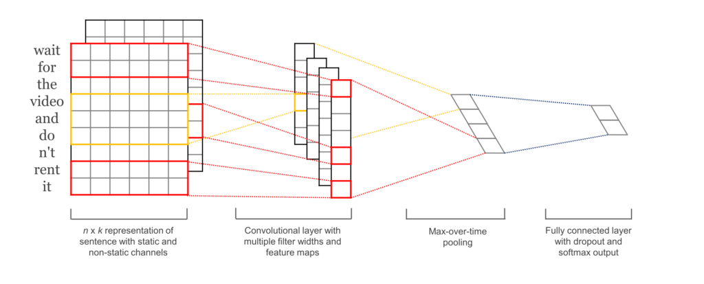
Convolutional Neural Networks (CNNs) are networks initially created for image-related tasks that can learn to capture specific features regardless of locality.

Convolutional Neural Networks는 지역성에 관계 없이 특정 feature를 포착하는 법을 배울 수 있는 이미지 관련 작업을 위해 처음 만들어진 network다.

For a more concrete example of that, imagine we use CNNs to distinguish pictures of Cars vs. pictures of Dogs. Since CNNs learn to capture features regardless of where these might be, the CNN will learn that cars have wheels, and every time it sees a wheel, regardless of where it is on the picture, that feature will activate.

좀 더 자세한 예를 들면, 자동차와 개의 사진을 구별하기 위해 CNN을 사용하는 것을 생각해보자. CNN은 사물이 어디에 있든 상관없이 feature를 포착하는 방법을 배우기 때문에 자동차가 바퀴를 가지고 있다는 것을 알게 될 것이고, 자동차가 사진의 어느 위치에 있는지와는 관계없이 바퀴를 볼 때마다 해당 feature를 활성화시킬 것이다.

In our particular case, it could capture a negative phrase such as "don't like" regardless of where it happens in the tweet.

• I don't like watching those types of films
• That's the one thing I really don't like.
• I saw the movie, and I don't like how it ended.

우리의 특별한 경우, tweet내에서 어느 위치인지는 상관 없이 "don't like"와 같은 부정적인 문장을 포착할 수 있었다.

• Source: wildml.com

2-2) LSTMs

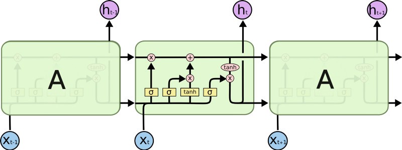
Long-Term Short Term Memory (LSTMs) are a type of network that has a memory that "remembers" previous data from the input and makes decisions based on that knowledge. These networks are more directly suited for written data inputs, since each word in a sentence has meaning based on the surrounding words (previous and upcoming words).

Long-Term Short Term Memory(LSTMs)는 input에서 이전 데이터를 "기억"하고, 그 지식을 바탕으로 결정을 내리는 메모리를 가진 네트워크의 일종이다. 이러한 network는 문장의 각 단어가 주변 단어(앞 단어, 뒷 단어)를 기반으로 의미를 가지기 때문에 written data input(글로 쓰여진 데이터)으로 더 직접적으로 적합하다.

In our particular case, it is possible that an LSTM could allow us to capture changing sentiment in a tweet. For example, a sentence such as: At first I loved it, but then I ended up hating it. has words with conflicting sentiments that would end-up confusing a simple Feed-Forward network. The LSTM, on the other hand, could learn that sentiments expressed towards the end of a sentence mean more than those expressed at the start.

우리의 특별한 경우, LSTM은 tweet에서 변하는 감정을 포착할 수 있도록 해준다. 예를 들어, 처음에는 좋아했지만 나중에는 싫어하게 되었다.와 같은 문장의 경우에는 단순한 Feed-Forward network를 혼란스럽게 할 수 있는 상반된 감정을 가진 단어들이 있다. 반면 LSTM은 문장의 끝에 표현된 감정이 처음에 표현된 감정보다 더 큰 의미가 있다는 것을 알 수 있다.

• Source: colah.github.io
         

3. Twitter Data

The Twitter data used for this particular experiment was a mix of two datasets:

이 특정 실험에 사용된 Twitter 데이터는 다음 두 개의 데이터셋을 혼합한 것이다.

• The University of Michigan Kaggle competition dataset.
• The Neik Sanders Twitter Sentiment Analysis corpus.

In total these datasets contain 1,578,627 labeled tweets.

이 전체 데이터셋에는 1,578,627개의 라벨링된 tweet들이 포함되어 있다.

4. CNN-LSTM Model

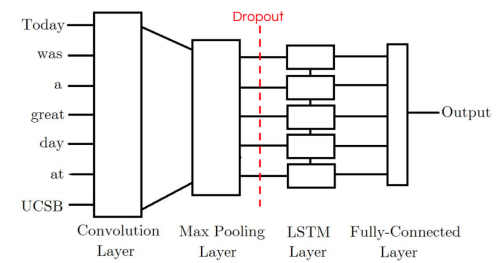
The first model I tried was the CNN-LSTM Model. Our CNN-LSTM model combination consists of an initial convolution layer which will receive word embeddings as input. Its output will then be pooled to a smaller dimension which is then fed into an LSTM layer. The intuition behind this model is that the convolution layer will extract local features and the LSTM layer will then be able to use the ordering of said features to learn about the input’s text ordering. In practice, this model is not as powerful as our other LSTM-CNN model proposed.

내가 처음 시도한 모델은 CNN-LSTM 모델이다. CNN-LSTM 모델 조합은 word embedding을 input으로 받을 수 있는 initial convolution layer로 이루어져 있다. CNN-LSTM 모델 조합의 output은 LSTM의 layer에 공급되는 것보다 더 작은 dimension으로 pooling될 것이다. 이 모델은 convolution layer가 local feature를 추출하고 그 다음 LSTM layer가 input 텍스트의 순서를 배우기 위해서 해당 feature의 순서를 사용할 수 있을 것이라고 생각했다. 실제로 이 모델은 제안된 다른 LSTM-CNN 모델보다 강력하지 않았다.

5. LSTM-CNN Model

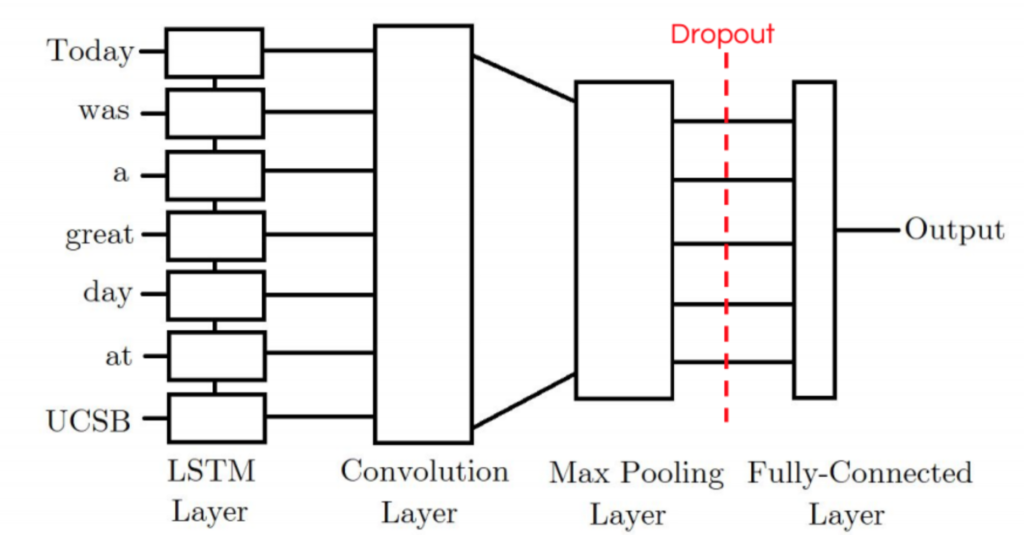
Our CNN-LSTM model consists of an initial LSTM layer which will receive word embeddings for each token in the tweet as inputs. The intuition is that its output tokens will store information not only of the initial token, but also any previous tokens; In other words, the LSTM layer is generating a new encoding for the original input. The output of the LSTM layer is then fed into a convolution layer which we expect will extract local features. Finally the convolution layer’s output will be pooled to a smaller dimension and ultimately outputted as either a positive or negative label.

CNN-LSTM 모델은 initial LSTM layer로 구성되며, LSTM layer는 tweet의 각 토큰에 대한 word embedding을 input으로 받는다. 이 모델은 output 토큰이 초기 토큰뿐만 아니라 이전 토큰의 정보를 저장할 것이라고 생각했다. 즉, LSTM layer는 원래 input에 대한 새로운 encoding을 생성한다. LSTM layer의 output은 local feature를 추출할 것이라고 기대하는 convolution layer에 제공한다. 마지막으로 convolution layer의 output은 작은 dimension으로 pooling되고 궁극적으로는 양수 또는 음수 라벨로 출력된다.

6. Results

We setup the experiment to use training sets of 10,000 tweets and testing sets of 2,500 labeled tweets. These training and testing sets contained equal amounts of negative and positive tweets. We re-did each test 5 times and reported on the average results of these tests.

실험에서 training셋으로 10,000개의 tweet과 testing셋으로 2,500개의 라벨링된 tweet을 사용했다. 이러한 training과 testing셋은 동일한 양의 부정적인 tweet과 긍정적인 tweet이 포함되도록 했다. 우리는 이러한 테스트를 5번 시도했고, 이 테스트의 평군 결과를 기록했다.

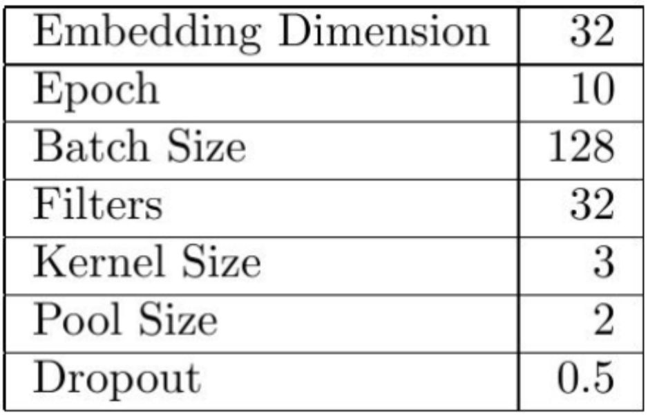
We used the following parameters which we fine-tuned through manual testing:

우리는 수동 테스트를 통해 다음과 같이 fine-tuned된 parameter를 사용했다.

The actual results were as follows:

실제 결과는 다음과 같았다.

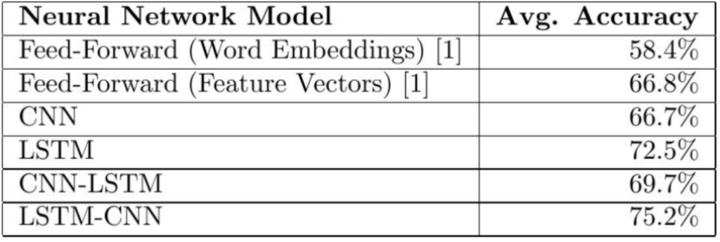
Our CNN-LSTM model achieved an accuracy of 3% higher than the CNN model, but 3.2% worse than the LSTM model. Meanwhile, our LSTM-CNN model performed 8.5% better than a CNN model and 2.7% better than an LSTM model.

CNN-LSTM 모델은 CNN 모델보다 3% 높은 정확도를 얻었지만 LSTM 모델보다 3.2% 낮은 정확도를 얻었다. 한편, LSTM-CNN 모델은 CNN 모델보다 8.5%, LSTM 모델보다 2.7% 더 나은 성능을 보였다.

These results seem to indicate that our initial intuition was correct, and that by combining CNNs and LSTMs we are able to harness both the CNN’s ability in recognizing local patterns, and the LSTM’s ability to harness the text’s ordering. However, the ordering of the layers in our models will play a crucial role on how well they perform.

이러한 결과는 우리의 처음 직감이 옳았음을 나타내며, CNN과 LSTM을 결합함으로써 CNN의 local 패턴 인식 능력과 LSTM의 텍스트 순서를 이용하는 능력을 사용할 수 있다는 것을 보여준다. 그리고 모델에서 layer의 순서는 각 layer 성능에 결정적인 역할을 할 것이다.

We believe that the 5.5% difference between our models is not coincidental. It seems that the initial convolutional layer of our CNN-LSTM is loosing some of the text’s order / sequence information. Thus, if the order of the convolutional layer does not really give us any information, the LSTM layer will act as nothing more than just a fully connected layer. This model seems to fail to harness the full capabilities of the LSTM layer and thus does not achieve its maximum potential. In fact, it even does worse than a regular LSTM model.

우리는 모델 사이의 5.5%의 차이가 우연이라고 생각하지 않는다. CNN-LSTM 모델의 initial convolutional layer가 텍스트의 순서 / sequence 정보를 일부 잃어버리고 있는 것처럼 보인다. 따라서, 만약 convolution layer의 순서가 실제로 우리에게 어떤 정보도 주지 않는다면, LSTM layer는 단지 fully connected layer 이상의 역할을 하지 않을 것이다. CNN-LSTM 모델은 LSTM layer의 모든 능력을 사용하지 못하지 때문에 최대로 능력을 달성하지 못한다. 사실, CNN-LSTM 모델은 일반 LSTM 모델보다 더 좋지 않다.

On the other hand, the LSTM-CNN model seems to be the best because its initial LSTM layer seems to act as an encoder such that for every token in the input there is an output token that contains information not only of the original token, but all other previous tokens. Afterwards, the CNN layer will find local patterns using this richer representation of the original input, allowing for better accuracy.

반면에, LSTM-CNN 모델은 모든 input token에 대해 원래 토큰 뿐만 아니라 모든 이전 토큰에 대한 정보를 포함한 output 토큰이 있어 LSTM layer가 encoder로 동작하기 때문에 LSTM-CNN 모델이 가장 적합한 것으로 보인다. 그 뒤에, CNN layer는 원래 input에 대한 풍부한 표현을 사용하여 local 패턴을 찾아 정확도를 높일 수 있다.

7. Further Observations

Some of the observations I made during the testing (and which are explained in much more detail on the paper):

테스트 중에 수행한 일부 관찰 사항(그리고 이것들은 논문에 훨씬 더 자세히 설명되어 있다.)

7-1) Learning Rates

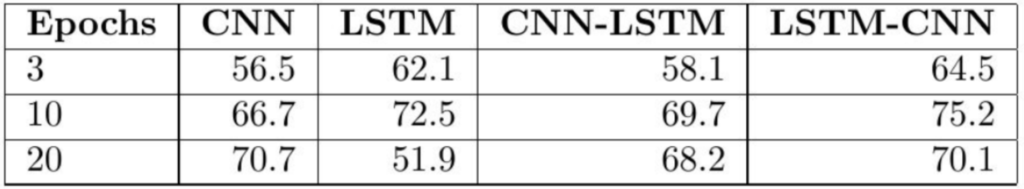
CNN & CNN-LSTM models need more epochs to learn and overfit less quickly, as opposed to LSTM & LSTM-CNN models.

CNN, CNN-LSTM 모델은 LSTM, LSTM-CNN 모델과는 달리 학습을 빠르게 하고 overfit을 줄이기 위해 더 많은 epoch이 필요하다.

7-2) Drop Rates

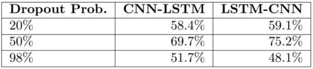
This wasn't so much of a surprise, but I did notice that it is very important to add a Dropout layer after any Convolutional layer in both the CNN-LSTM and LSTM-CNN models.

이것은 많이 놀라운 것은 아니었지만, CNN-LSTM 모델과 LSTM-CNN 모델 둘 다 convolutional layer뒤에 dropout layer를 추가하는 것이 매우 중요하다는 것을 알아차렸다.

(Note: in this case Dropout Prob. is how likely we are to drop a random input.)

(참고: 이 경우, Dropout Prob.는 random input을 얼마나 뺄 것인지에 대한 비율이다.)

7-3) Pre-Trained Word Embeddings

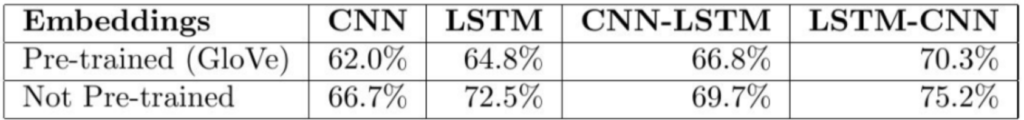
I attempted to use pre-trained word embeddings, as opposed to having the system learn the word embeddings form our data. Surprisingly using these pre-trained GloVe word embeddings gave us worst accuracy. I believe this might be due to the fact that twitter data contains multiple misspellings, emojis, mentions, and other twitter-specific text irregularities that weren't taken into consideration when building the GloVe embeddings.

나는 우리의 데이터에서 word embedding을 학습하는 시스템을 갖는 것과 반대로, pre-trained word embeddings을 사용하려고 시도했다. 놀랍게도, pre-trained GloVe word embedding은 최악의 정확도를 얻었다. 나는 다수의 철자 오류, 이모티콘, 멘션 및 기타 twitter 관련 텍스트 불규칙성을 가지고 있는 twitter 데이터가 GloVe embedding을 구축할 때 고려되지 않았기 때문일지도 모른다고 생각한다.

8. Conclusions & Future Work

In terms of future work, I would like to test other types of LSTMs (for example Bi-LSTMs) and see what effects this has on the accuracy of our systems. It would also be interesting to find a better way to deal with misspellings or other irregularities found on twitter language. I believe this could be achieved by building Twitter specific word-embeddings. Lastly, it would be interesting to make use of Twitter specific features, such as # of retweets, likes, etc. to feed along the text data.

향후 작업적인 측면에서, 다른 종류의 LSTMs(예를들면 Bi-LSTMs)을 테스트하여 이것이 우리 시스템의 정확도에 어떤 영향을 미치는지 확인하고 싶다. 또한 twitter 언어에서 발견되는 철자 오류나 기타 불규칙성에 대한 더 좋은 방법을 찾는 것도 흥미로울 것이다. 나는 Twitter만의 word embedding을 구축할 수 있을 것이라고 생각한다. 마지막으로, 텍스트 데이터를 feed(추가)하기 위해 retweet을 위한 #, 좋아요 등과 같은 twitter 특정 feature를 이용하는 것도 재미있을 것이다.

On a personal note, this project was mainly intended as an excuse to further understand CNN and LSTM models, along with experimenting with Tensorflow. Moreover, I was happy to see that these two models did much better than our previous (naive) attempts.

개인적으로 이 프로젝튼 Tensorflow를 실험하면서 CNN과 LSTM 모델을 더 이해하기 위한 핑계였다. 게다가 나는 CNN과 LSTM 모델이 이전의 시도(naive)보다 훨씬 좋은 것을 보고 기뻤다.

As always, the source code and paper are publicly available: paper & code. If you have any questions or comments feel free to reach out. Happy coding! 🙂

항상 그렇듯이, 소스 코드와 논문은 공개적으로 사용 가능하다: 논문 & 코드. 질문이나 의견이 있으면 언제든지 연락해라. 즐거운 코딩해라!

자주 사용하는 Github Markdown 정리

Text

• 밑줄

<ins>underline</ins>

Images

• Github 레포 주소로 지정

![image.png](https://github.com/tmfdk333/repo-name/blob/master/image_path.png)

• 이미지 크기 지정

<img src=https://github.com/tmfdk333/repo-name/blob/master/image_path.png width=560>

Emoji Cheat Sheet

• For Repository

• For Article

Mac OS X Mojave 10.14.3

RaspberryPI2에 LCD Driver 설치하기(deb to rpm)

• Debian 기반의 Driver 설치 스크립트를 Redhat 기반에 맞게 변경

[1] Install Package

• xserver-xorg-input-evdev(deb) → xorg-x11-drv-evdev, xorg-x11-drv-evdev-devel(rpm)
• xinput-calibrator_0.7.5-1_armhf(deb) → xorg-x11-drv-synaptics, xorg-x11-drv-synaptics-devel(rpm)
• bcm_host.h

yum install -y xorg-x11-drv-evdev xorg-x11-drv-evdev-devel
yum install -y xorg-x11-drv-synaptics xorg-x11-drv-synaptics-devel
yum install -y raspberrypi-vc-libs raspberrypi-vc-libs-devel 
cp -rf /usr/share/X11/xorg.conf.d/10-evdev.conf /usr/share/X11/xorg.conf.d/45-evdev.conf
cp -rf /usr/include/vc/* /usr/include/ 

[2] Build

yum install -y gcc gcc-c++ cmake make git
git clone https://github.com/waveshare/LCD-show.git
cd LCD-show/rpi-fbcp/build/

• CMakeCache.txt 파일 수정 & cmake(line: 169, 172, 182, 245)

# Edit "/home/pi" to "/home/tmfdk333"
:%s/\/home\/pi/\/home\/tmfdk333/g
cmake ..

• CMakeFiles/fbcp.dir/link.txt 파일 수정 & make & install

# Edit line 1 "/opt/vc/lib" to "/usr/lib/vc"
:%s/\/opt\/vc\/lib/\/usr\/lib\/vc/g
make 
install fbcp /usr/local/bin/fbcp

[3] Run Script

cd ../../
sudo cp -rf ./etc/rc.local /etc/rc.local
# "LCD configure 0"
sudo cp -rf ./etc/X11/xorg.conf.d/99-calibration.conf-5  /usr/share/X11/xorg.conf.d/99-calibration.conf
sudo cp ./boot/config-5.txt /boot/config.txt
# !!SKIP IF GNOME!!
sudo cp -rf ./usr/share/X11/xorg.conf.d/99-fbturbo.conf-HDMI /usr/share/X11/xorg.conf.d/99-fbturbo.conf 

• cmdline.txt 파일 수정 & reboot

# -b /dev/mmcblk0p7 else
:%s/mmcblk0p2/mmcblk0p3/g
:%s/logo.nologo//g
sudo cp ./cmdline.txt /boot/
reboot

[4] Reference

• waveshare-wiki/5inch HDMI LCD, waveshare/LCD-show
• Package: xserver-xorg-input-evdev : X.Org X server -- evdev input driver
  • xorg-x11-drv-evdev.armv7hl : Xorg X11 evdev input driver
  • xorg-x11-drv-evdev-devel.armv7hl : Xorg X11 evdev input driver development package.
• xinput calibrator : A generic touchscreen calibration program for X.Org
  • xorg-x11-drv-synaptics.armv7hl : Xorg X11 Synaptics touchpad input driver
  • xorg-x11-drv-synaptics-devel.armv7hl : Xorg X11 synaptics input driver
• cc Compiler Options
• failed to Cross compile Qt 5.6 on RPi 2 (fatal error: bcm_host.h: No such file or directory)
• The Kernel Command Line

RaspberryPi2에 CentOS7 설치하기

Mac OS X Mojave 10.14.3

[1] Download Image

• Gnome(GUI) - CentOS Download > Genome image for Raspberrypi2/3
• Minimal(Only CLI) - CentOS Download > Minimal image for RaspberryPi 2/3

[2] Unmount Disk

diskutil unmountDisk /dev/disk2

[3] Make Bootable MicroSD Card

# Gnome
xzcat CentOS-Userland-7-armv7hl-RaspberryPI-GNOME-1810-sda.raw.xz | pv | sudo dd of=/dev/disk2 bs=64m
# Minimal
xzcat CentOS-Userland-7-armv7hl-RaspberryPI-Minimal-1810-sda.raw.xz | pv | sudo dd of=/dev/disk2 bs=64m

[4] Expand the RootFS

/usr/bin/rootfs-expand

# Before
/dev/disk2 (external, physical):
   #:                       TYPE NAME                    SIZE       IDENTIFIER
   0:     FDisk_partition_scheme                        *64.1 GB    disk2
   1:             Windows_FAT_32 NO NAME                 700.4 MB   disk2s1
   2:                 Linux_Swap                         511.7 MB   disk2s2
   3:                      Linux                         1.5 GB     disk2s3
# After
/dev/disk2 (external, physical):
   #:                       TYPE NAME                    SIZE       IDENTIFIER
   0:     FDisk_partition_scheme                        *64.1 GB    disk2
   1:             Windows_FAT_32 NO NAME                 700.4 MB   disk2s1
   2:                 Linux_Swap                         511.7 MB   disk2s2
   3:                      Linux                         62.9 GB    disk2s3

[5] Reference

• RaspberryPi 3 with CentOS-7
• RaspberryPi 3 model B+ CentOS 7 image
• SpecialInterestGroup>AltArch>armhfp
• How to Erase a Disk from Command Line in Mac OS X
• How do you monitor the progress of dd?