M²E³D discovers equations, models and correlations underpinning experimental data.

It builds on the fantastic PySR and fvGP libraries to build a user-facing package offering:

• Discovery of symbolic closed-form equations that model multiple responses.
• Efficient parameter sampling for planning experimental / simulational campaigns.
• System multi-response uncertainty quantification - and specifically targeting high-variance parameter regions.
• Automatic parallelisation of complex user simulation scripts on OS Processes and distributed supercomputers.
• Interactive plotting of responses, uncertainties, discovered model outputs.
• Language-agnostic saving of results found.

M²E³D was developed to discover physical laws and correlations in chemical engineering, but it is data-agnostic - and works with both simulated and experimental results in any domain.

How does a system behave under different conditions? E.g. drag force acting on a sphere for different flow velocities. M²E³D can explore multiple responses in one of two ways:

1. Locally / manually: running experiments / simulations, then feeding results back to MED.
2. Massively parallel: for complex simulations that can be launched in Python, MED can automatically change simulation parameters and run them in parallel on OS processes (locally) or SLURM jobs (distributed clusters).

Here is a minimal example showing the main interface to the medeq.MED object. For automatic parallelisation and other features, see the docs.

import medeq
import numpy as np


# Create DataFrame of MED free parameters and their bounds
parameters = medeq.create_parameters(
    ["velocity", "viscosity", "radius"],
    minimums = [-9, -9, -9],
    maximums = [10, 10, 10],
)


def instrument(x):
    '''Example unknown "experimental response" - a complex non-convex function.
    '''
    return x[0] * np.sin(0.5 * x[1]) + np.cos(1.1 * x[2])


# Create MED object, keeping track of free parameters, samples and results
med = medeq.MED(parameters)

# Initial parameter sampling
med.sample(24)
med.evaluate(instrument)

# New sampling, targeting most uncertain parameter regions
med.sample(16)
med.evaluate(instrument)

# Add previous / manually-evaluated responses
med.augment([[0, 0, 0]], [1])

# Save all results to disk - you can load them on another machine
med.save("med_results")

# Discover underlying equation; tell MED what operators it may use
med.discover(
    binary_operators = ["+", "-", "*", "/"],
    unary_operators = ["cos"],
)

# Plot interactive 2D slices of responses and uncertainties
med.plot_gp()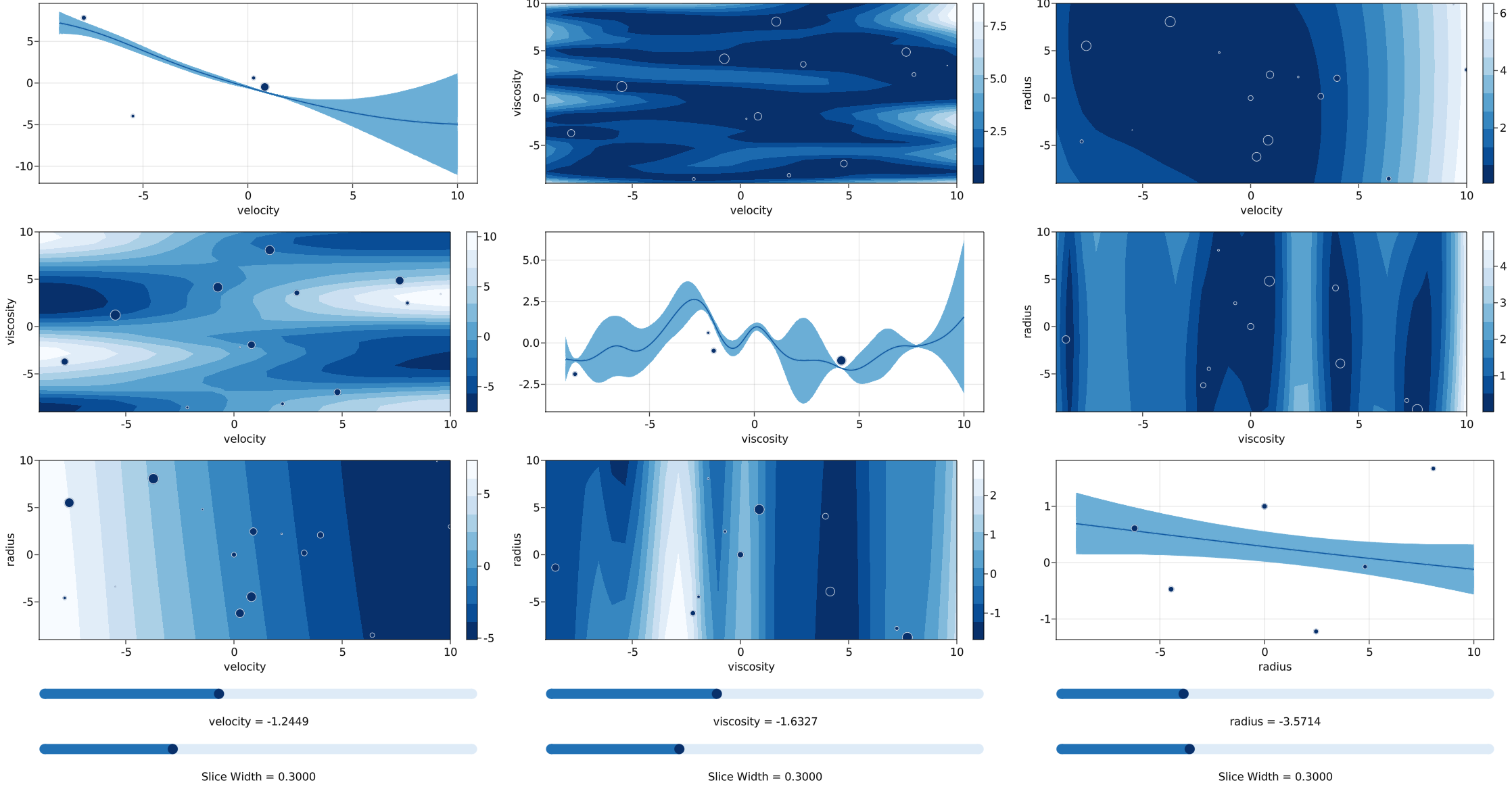

Here are the equations found by SymbolicRegression.jl at various complexity levels:

==============================
Hall of Fame:
-----------------------------------------
Complexity  Loss       Score     Equation
1           1.656e+01  1.025e-07  -0.19632196
2           1.626e+01  1.812e-02  cos(radius)
3           1.541e+01  5.332e-02  (-0.20152433 * velocity)
4           1.227e+01  2.278e-01  (velocity * cos(velocity))
6           8.668e+00  1.739e-01  (velocity * cos(-1.0899653 * velocity))
8           4.988e-01  1.428e+00  (velocity * cos(1.5935777 + (-0.50125474 * viscosity)))
10          4.946e-01  4.271e-03  ((-1.016915 * velocity) * cos(7.8330894 + (0.5005289 * viscosity)))
11          1.241e-01  1.383e+00  (cos(radius) + (velocity * cos(1.5515859 + (-0.49880704 * viscosity))))
13          0.000e+00  1.151e+01  (cos(1.1000026 * radius) + (velocity * cos(1.5707898 + (-0.50000036 * viscosity))))

Note how it discovered the sin(x) term as cos(1.57 + x).

Before the medeq library is published to PyPI, you can install it directly from this GitHub repository:

$> pip install git+https://github.com/uob-positron-imaging-centre/MED

Alternatively, you can download all the code and run pip install . inside its directory:

$> git clone https://github.com/uob-positron-imaging-centre/MED
$> cd MED
$MED> pip install .

If you would like to modify the source code and see your changes without reinstalling the package, use the -e flag for a development installation:

$MED> pip install -e .

To discover underlying equations and see interactive plots of system responses, uncertainties and model outputs, you need to install Julia (a beautiful, high-performance programming language) on your system and the PySR library:

1. Install Julia manually (see Julia downloads, version >=1.8 is recommended).
2. import medeq; medeq.install()

... and discover underlying physical laws / correlations.

Exploring systems responses can be done in one of two ways:

1. Locally / manually: running experiments / simulations, then feeding results back to MED.
2. Massively parallel: for complex simulations that can be launched in Python, MED can automatically change simulation parameters and run them in parallel on OS processes (locally) or SLURM jobs (distributed clusters).

A typical local workflow is:

1. Define free parameters to explore as a pd.DataFrame - you can use the medeq.create_parameters function for this.

>>> import medeq
>>> parameters = medeq.create_parameters(
>>>     ["A", "B"],
>>>     minimums = [-5., -5.],
>>>     maximums = [10., 10.],
>>> )
>>> print(parameters)
   value  min   max
A    2.5 -5.0  10.0
B    2.5 -5.0  10.0

2. Create a medeq.MED object and generate samples (i.e. parameter combinations) to evaluate - the default sampler covers the parameter space as efficiently as possible, taking previous results into account; use the MED.sample(n) method to get n samples to try.

>>> med = medeq.MED(parameters, seed = 42)
>>> print(med)
MED(seed=42)
---------------------------------------
parameters =
     value  min   max
  A    2.5 -5.0  10.0
  B    2.5 -5.0  10.0
response_names =
  None
---------------------------------------
sampler =   DVASampler(d=2, seed=42)
samples =   np.ndarray[(0, 2), float64]
responses = NoneType
epochs =    list[0, tuple[int, int]]

>>> med.sample(5)
array([[-3.33602115, -0.45639296],
       [ 5.55496225,  5.554965  ],
       [ 2.72771903, -3.48852585],
       [-0.45639308,  8.33602069],
       [ 8.48852568,  2.27228172]])

3. For a local / offline workflow, these samples can be evaluated in one of two ways:

   • Evaluate samples manually, offline - i.e. run experiments, simulations, etc. and feed them back to MED.
   • Let MED evaluate a simple Python function / model.

>>> # Evaluate samples manually - run experiments, simulations, etc.
>>> to_evaluate = med.queue
>>> responses = [1, 2, 3, 4, 5]
>>> med.evaluate(responses)
>>>
>>> # Or evaluate simple Python function / model
>>> def instrument(sample):
>>>     return sample[0] + sample[1]
>>>
>>> med.evaluate(instrument)
>>> med.results
          A         B  variance   response
0 -3.336021 -0.456393  0.037924  -3.792414
1  5.554962  5.554965  0.111099  11.109927
2  2.727719 -3.488526  0.007608  -0.760807
3 -0.456393  8.336021  0.078796   7.879628
4  8.488526  2.272282  0.107608  10.760807

For a massively parallel workflow, e.g. using a complex simulation, all you need is a standalone Python script that:

• Defines its free parameters between two # MED PARAMETERS START / END directives.
• Runs the simulation in any way - define simulation inline, launch it on a supercomputer and collect results, etc.
• Defines a variable "response" for the simulated output of interest - either as a single number or a list of numbers (multi-response), or a dictionary with names for each response.

Here is a simple example of a MED script:

# In file `simulation_script.py`

# MED PARAMETERS START
import medeq

parameters = medeq.create_parameters(
    ["A", "B", "C"],
    [-5., -5., -5.],
    [10., 10., 10.],
)
# MED PARAMETERS END

# Run simulation in any way, locally, on a supercomputer and collect
# results - then define the variable `response` (float or list[float])
values = parameters["value"]
response = values["A"]**2 + values["B"]**2

If you have previous, separate experimental data, you can MED.augment the dataset of responses:

>>> # Augment dataset of responses with historical data
>>> samples = [
>>>     [1, 1],
>>>     [2, 2],
>>>     [1, 2],
>>> ]
>>>
>>> responses = [1, 2, 3]
>>> med.augment(samples, responses)

And now discover underlying equations!

>>> med.discover(binary_operators = ["+", "*"])
Hall of Fame:
-----------------------------------------
Complexity  Loss       Score     Equation
1           2.412e+01  5.296e-01  B
3           0.000e+00  1.151e+01  (A + B)

You are more than welcome to contribute to this package in the form of library improvements, documentation or helpful examples; please submit them either as:

• GitHub issues.
• Pull requests.
• Email me at [email protected].

The authors gratefully acknowledge the following funding, without which M²E³D would not have been possible:

M²E³D: Multiphase Materials Exploration via Evolutionary Equation Discovery
Royce Materials 4.0 Feasibility and Pilot Scheme Grant, £57,477

If you use this library in your research, you are kindly asked to cite:

Nicusan, A., & Windows-Yule, K. (2022). M2E3D: Multiphase Materials Exploration via Evolutionary Equation Discovery (Version 0.1.0) [Computer software]

This library would not have been possible without the excellent PySR and fvGP packages, which form the very core of the symbolic regression and Gaussian Process engines. If you use medeq in your published work, please also cite:

Miles Cranmer. (2020). MilesCranmer/PySR v0.2 (v0.2). Zenodo. https://doi.org/10.5281/zenodo.4041459

Marcus Michael Noack, Ian Humphrey, elliottperryman, Ronald Pandolfi, & MarcusMichaelNoack. (2022). lbl-camera/fvGP: (3.2.11). Zenodo. https://doi.org/10.5281/zenodo.6147361

The medeq library is published under the GPL v3.0 license.