Sounds like time traveling or some kind of future technic, however, it is not. Dynamic Time Warping is used to compare the similarity or calculate the distance between two arrays or time series with different length.
Suppose we want to calculate the distance of two equal-length arrays:
a = [1, 2, 3]
b = [3, 2, 2]
How to do that? One obvious way is to match up a and b in 1-to-1 fashion and sum up the total distance of each component. This sounds easy, but what if a and b have different lengths?
a = [1, 2, 3]
b = [2, 2, 2, 3, 4]
How to match them up? Which should map to which? To solve the problem, there comes dynamic time warping. Just as its name indicates, to warp the series so that they can match up.
Before digging into the algorithm, you might have the question that is it useful? Do we really need to compare the distance between two unequal-length time series?
Yes, in a lot of scenarios DTW is playing a key role.
One use case is to detect the sound pattern of the same kind. Suppose we want to recognise the voice of a person by analysing his sound track, and we are able to collect his sound track of saying Hello in one scenario. However, people speak in the same word in different ways, what if he speaks hello in a much slower pace like Heeeeeeelloooooo , we will need an algorithm to match up the sound track of different lengths and be able to identify they come from the same person.

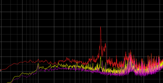
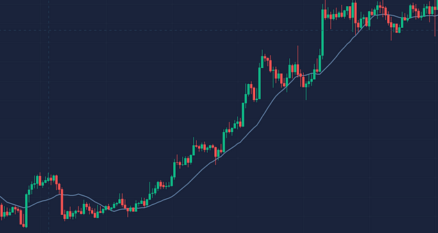
In a stock market, people always hope to be able to predict the future, however using general machine learning algorithms can be exhaustive, as most prediction task requires test and training set to have the same dimension of features. However, if you ever speculate in the stock market, you will know that even the same pattern of a stock can have very different length reflection on klines and indicators.

A concise explanation of DTW from wiki,
In time series analysis, dynamic time warping (DTW) is one of the algorithms for measuring similarity between two temporal sequences, which may vary in speed. DTW has been applied to temporal sequences of video, audio, and graphics data --- indeed, any data that can be turned into a linear sequence can be analysed with DTW.
The idea to compare arrays with different length is to build one-to-many and many-to-one matches so that the total distance can be minimised between the two.
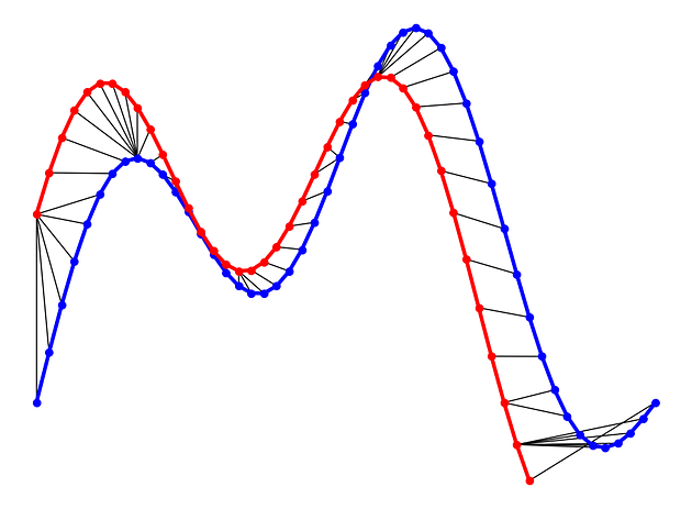
Suppose we have two different arrays red and blue with different length:

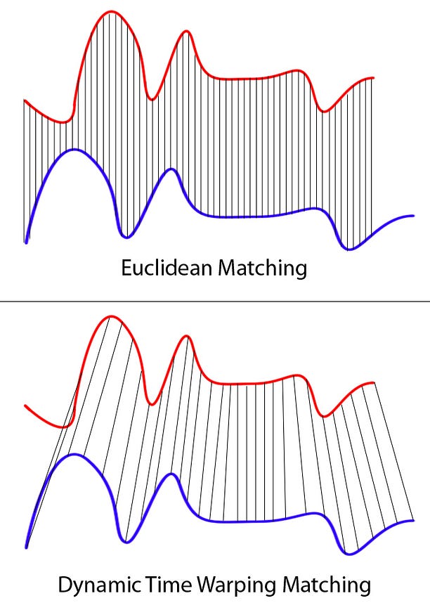
Clearly these two series follow the same pattern, but the blue curve is longer than the red. If we apply the one-to-one match, shown in the top, the mapping is not perfectly synced up and the tail of the blue curve is being left out.
DTW overcomes the issue by developing a one-to-many match so that the troughs and peaks with the same pattern are perfectly matched, and there is no left out for both curves(shown in the bottom top).
In general, DTW is a method that calculates an optimal match between two given sequences (e.g. time series) with certain restriction and rules(comes from wiki):
- Every index from the first sequence must be matched with one or more indices from the other sequence and vice versa
- The first index from the first sequence must be matched with the first index from the other sequence (but it does not have to be its only match)
- The last index from the first sequence must be matched with the last index from the other sequence (but it does not have to be its only match)
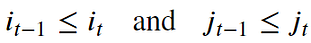
- The mapping of the indices from the first sequence to indices from the other sequence must be monotonically increasing, and vice versa, i.e. if
j > iare indices from the first sequence, then there must not be two indicesl > kin the other sequence, such that indexiis matched with indexland indexjis matched with indexk, and vice versa
The optimal match is denoted by the match that satisfies all the restrictions and the rules and that has the minimal cost, where the cost is computed as the sum of absolute differences, for each matched pair of indices, between their values.
To summarise is that head and tail must be positionally matched, no cross-match and no left out.
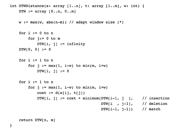
The implementation of the algorithm looks extremely concise:

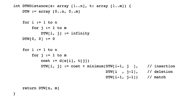
where DTW[i, j] is the distance between s[1:i] and t[1:j] with the best alignment.
The key lies in:
DTW[i, j] := cost + minimum(DTW[i-1, j ],
DTW[i , j-1],
DTW[i-1, j-1])
Which is saying that the cost of between two arrays with length i and j equals the distance between the tails + the minimum of cost in arrays with length *i-1, j* , *i, j-1* , and *i-1, j-1* .
Put it in python would be:
Example:

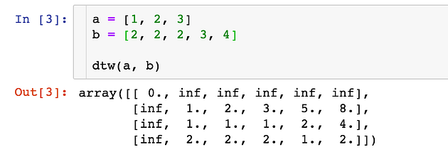
The distance between a and b would be the last element of the matrix, which is 2.
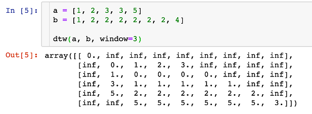
One issue of the above algorithm is that we allow one element in an array to match an unlimited number of elements in the other array(as long as the tail can match in the end), this would cause the mapping to bent over a lot, for example, the following array:
a = [1, 2, 3]
b = [1, 2, 2, 2, 2, 2, 2, 2, ..., 5]
To minimise the distance, the element 2 in array a would match all the 2 in array b , which causes an array b to bent severely. To avoid this, we can add a window constraint to limit the number of elements one can match:

The key difference is that now each element is confined to match elements in range i --- w and i + w . The w := max(w, abs(n-m)) guarantees all indices can be matched up.
The implementation and example would be:

There is also contributed packages available on Pypi to use directly. Here I demonstrate an example using fastdtw:
It gives you the distance of two lists and index mapping(the example can extend to a multi-dimension array).
Lastly, you can check out the implementation here.
Reference:
[1] https://databricks.com/blog/2019/04/30/understanding-dynamic-time-warping.html
[2] https://en.wikipedia.org/wiki/Dynamic_time_warping
| | | | | DTW algorithm | | | | | | | | Dynamic time warping (DTW) is a time series alignment algorithm developed originally for speech recognition^(1)^. It aims at aligning two sequences of feature vectors by warping the time axis iteratively until an optimal match (according to a suitable metrics) between the two sequences is found.
Consider two sequences of feature vectors:
The two sequences can be arranged on the sides of a grid, with one on the top and the other up the left hand side. Both sequences start on the bottom left of the grid.
Inside each cell a distance measure can be placed, comparing the corresponding elements of the two sequences. To find the best match or alignment between these two sequences one need to find a path through the grid which minimizes the total distance between them. The procedure for computing this overall distance involves finding all possible routes through the grid and for each one compute the overall distance. The overall distance is the minimum of the sum of the distances between the individual elements on the path divided by the sum of the weighting function. The weighting function is used to normalise for the path length. It is apparent that for any considerably long sequences the number of possible paths through the grid will be very large. The major optimisations or constraints of the DTW algorithm arise from the observations on the nature of acceptable paths through the grid:
-
Monotonic condition: the path will not turn back on itself, both the i and j indexes either stay the same or increase, they never decrease.
-
Continuity condition: the path advances one step at a time. Both i and j can only increase by at most 1 on each step along the path.
-
Boundary condition: the path starts at the bottom left and ends at the top right.
-
Warping window condition: a good path is unlikely to wander very far from the diagonal. The distance that the path is allowed to wander is the window width.
-
Slope constraint condition: The path should not be too steep or too shallow. This prevents short sequences matching too long ones. The condition is expressed as a ratio p/q where p is the number of steps allowed in the same (horizontal or vertical) direction. After p steps in the same direction is not allowed to step further in the same direction before stepping at least q time in the diagonal direction.
The foregoing constraints allow to restrict the moves that can be made from any point in the path and so limit the number of paths that need to be considered. The power of the DTW algorithm is in the fact that instead finding all possible routes through the grid which satisfy the above conditions, the DTW algorithm works by keeping track of the cost of the best path to each point in the grid. During the calculation process of the DTW grid it is not known which path is minimum overall distance path, but this can be traced back when the end point is reached.
A detailed technical presentation of the DTW algorithm can be downloaded from here DTW algorithm.
|
ynamic Time Warping (DTW) is a way to compare two -usually temporal- sequences that do not sync up perfectly. It is a method to calculate the optimal matching between two sequences. DTW is useful in many domains such as speech recognition, data mining, financial markets, etc. It's commonly used in data mining to measure the distance between two time-series.
In this post, we will go over the mathematics behind DTW. Then, two illustrative examples are provided to better understand the concept. If you are not interested in the math behind it, please jump to examples.
Let's assume we have two sequences like the following:
𝑋=𝑥[1], 𝑥[2], ..., x[i], ..., x[n]
Y=y[1], y[2], ..., y[j], ..., y[m]
The sequences 𝑋 and 𝑌 can be arranged to form an 𝑛-by-𝑚 grid, where each point (𝑖, j) is the alignment between 𝑥[𝑖] and 𝑦[𝑗].
A warping path 𝑊 maps the elements of 𝑋 and 𝑌 to minimize the distance between them. 𝑊 is a sequence of grid points (𝑖, 𝑗). We will see an example of the warping path later.
The Optimal path to (𝑖_𝑘, 𝑗_𝑘) can be computed by:


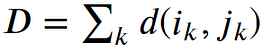
where 𝑑 is the Euclidean distance. Then, the overall path cost can be calculated as

The warping path is found using a dynamic programming approach to align two sequences. Going through all possible paths is "combinatorically explosive" [1]. Therefore, for efficiency purposes, it's important to limit the number of possible warping paths, and hence the following constraints are outlined:
- Boundary Condition: This constraint ensures that the warping path begins with the start points of both signals and terminates with their endpoints.


- Monotonicity condition: This constraint preserves the time-order of points (not going back in time).

- Continuity (step size) condition: This constraint limits the path transitions to adjacent points in time (not jumping in time).


In addition to the above three constraints, there are other less frequent conditions for an allowable warping path:
- Warping window condition: Allowable points can be restricted to fall within a given warping window of width 𝜔 (a positive integer).

- Slope condition: The warping path can be constrained by restricting the slope, and consequently avoiding extreme movements in one direction.
An acceptable warping path has combinations of chess king moves that are:
- Horizontal moves: (𝑖, 𝑗) → (𝑖, 𝑗+1)
- Vertical moves: (𝑖, 𝑗) → (𝑖+1, 𝑗)
- Diagonal moves: (𝑖, 𝑗) → (𝑖+1, 𝑗+1)
Let's import all python packages we need.
import pandas as pd
import numpy as np# Plotting Packages
import matplotlib.pyplot as plt
import seaborn as sbn# Configuring Matplotlib
import matplotlib as mpl
mpl.rcParams['figure.dpi'] = 300
savefig_options = dict(format="png", dpi=300, bbox_inches="tight")# Computation packages
from scipy.spatial.distance import euclidean
from fastdtw import fastdtw
Let's define a method to compute the accumulated cost matrix D for the warp path. The cost matrix uses the Euclidean distance to calculate the distance between every two points. The methods to compute the Euclidean distance matrix and accumulated cost matrix are defined below:
In this example, we have two sequences x and y with different lengths.
x = [3, 1, 2, 2, 1]
y = [2, 0, 0, 3, 3, 1, 0]
We cannot calculate the Euclidean distance between x and y since they don't have equal lengths.

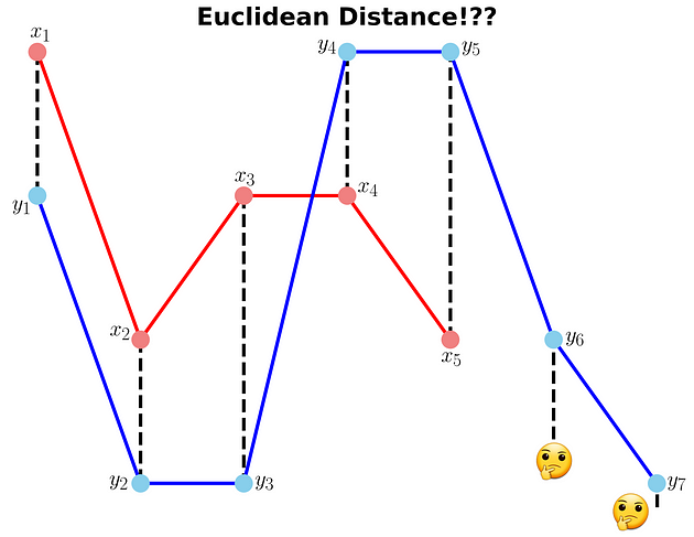
Example 1: Euclidean distance between x and y (is it possible? 🤔) (Image by Author)
Many Python packages calculate the DTW by just providing the sequences and the type of distance (usually Euclidean). Here, we use a popular Python implementation of DTW that is FastDTW which is an approximate DTW algorithm with lower time and memory complexities [2].
dtw_distance, warp_path = fastdtw(x, y, dist=euclidean)
Note that we are using SciPy's distance function Euclidean that we imported earlier. For a better understanding of the warp path, let's first compute the accumulated cost matrix and then visualize the path on a grid. The following code will plot a heatmap of the accumulated cost matrix.
cost_matrix = compute_accumulated_cost_matrix(x, y)
Example 1: Python code to plot (and save) the heatmap of the accumulated cost matrix

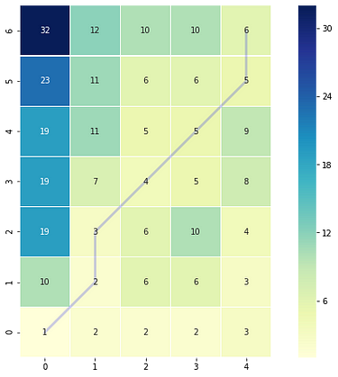
Example 1: Accumulated cost matrix and warping path (Image by Author)
The color bar shows the cost of each point in the grid. As can be seen, the warp path (blue line) is going through the lowest cost on the grid. Let's see the DTW distance and the warping path by printing these two variables.
DTW distance: 6.0
Warp path: [(0, 0), (1, 1), (1, 2), (2, 3), (3, 4), (4, 5), (4, 6)]
The warping path starts at point (0, 0) and ends at (4, 6) by 6 moves. Let's also calculate the accumulated cost most using the functions we defined earlier and compare the values with the heatmap.
cost_matrix = compute_accumulated_cost_matrix(x, y)
print(np.flipud(cost_matrix)) # Flipping the cost matrix for easier comparison with heatmap values!>>> [[32. 12. 10. 10. 6.]
[23. 11. 6. 6. 5.]
[19. 11. 5. 5. 9.]
[19. 7. 4. 5. 8.]
[19. 3. 6. 10. 4.]
[10. 2. 6. 6. 3.]
[ 1. 2. 2. 2. 3.]]
The cost matrix is printed above has similar values to the heatmap.
Now let's plot the two sequences and connect the mapping points. The code to plot the DTW distance between x and y is given below.
Example 1: Python code to plot (and save) the DTW distance between x and y

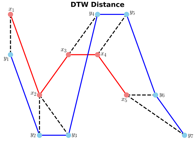
Example 1: DTW distance between x and y (Image by Author)
In this example, we will use two sinusoidal signals and see how they will be matched by calculating the DTW distance between them.
Example 2: Generate two sinusoidal signals (x1 and x2) with different lengths
Just like Example 1, let's calculate the DTW distance and the warp path for *x1 *and *x2 *signals using FastDTW package.
distance, warp_path = fastdtw(x1, x2, dist=euclidean)
Example 2: Python code to plot (and save) the DTW distance between x1 and x2

Example 2: DTW distance between x1 and x2 (Image by Author)
As can be seen in above figure, the DTW distance between the two signals is particularly powerful when the signals have similar patterns. The extrema (maximum and minimum points) between the two signals are correctly mapped. Moreover, unlike Euclidean distance, we may see many-to-one mapping when DTW distance is used, particularly if the two signals have different lengths.
You may spot an issue with dynamic time warping from the figure above. Can you guess what it is?
The issue is around the head and tail of time-series that do not properly match. This is because the DTW algorithm cannot afford the warping invariance for at the endpoints. In short, the effect of this is that a small difference at the sequence endpoints will tend to contribute disproportionately to the estimated similarity[3].
DTW is an algorithm to find an optimal alignment between two sequences and a useful distance metric to have in our toolbox. This technique is useful when we are working with two non-linear sequences, particularly if one sequence is a non-linear stretched/shrunk version of the other. The warping path is a combination of "chess king" moves that starts from the head of two sequences and ends with their tails.
Find out why DTW is a very useful technique to compare two or more time series signals and add it to your time series analysis toolbox!!
1. Introduction
In this world which is getting dominated by Internet of Things (IoT), there is an increasing need to understand signals from devices installed in households, shopping malls, factories and offices. For example, any voice assistant detects, authenticates and interprets commands from humans even if it is slow or fast. Our voice tone tends to be different during different times of the day. In the early morning after we get up from bed, we interact with a slower, heavier and lazier tone compared to other times of the day. These devices treat the signals as time series and compare the peaks, troughs and slopes by taking into account the varying lags and phases in the signals to come up with a similarity score. One of the most common algorithms used to accomplish this is Dynamic Time Warping (DTW). It is a very robust technique to compare two or more Time Series by ignoring any shifts and speed.
As part of Walmart Real Estate team, I am working on understanding the energy consumption pattern of different assets like refrigeration units, dehumidifiers, lighting, etc. installed in the retail stores.This will help in improving quality of data collected from IoT sensors, detect and prevent faults in the systems and improve energy consumption forecasting and planning. This analysis involves time series of energy consumption during different times of a day i.e. different days of a week, weeks of a month and months of a year. Time series forecasting often gives bad predictions when there is sudden shift in phase of the energy consumption due to unknown factors. For example if the defrost schedule, items refresh routine for a refrigeration unit, or weather changes suddenly and are not captured to explain the phase shifts of energy consumption, it is important to detect these change points.
In the example below, the items refresh routine of a store has shifted by 2 hours on Tuesday leading the shift in peak energy consumption of refrigeration units and this information was not available to us for many such stores.


The peak at 2 am got shifted to 4 am. DTW when run recursively for consecutive days can identify the cases for which phase shift occurred without much change in shape of signals.


The training data can be restricted to Tuesday onwards to improve the prediction of energy consumption in future in this case as phase shift was detected on Tuesday. The setup improved the predictions substantially ( > 50%) for the stores for which the reason of shift was not known. This was not possible by traditional ways of one to one comparison of signals.
In this blog, I will explain how DTW algorithm works and throw some light on the calculation of the similarity score between two time series and its implementation in python. Most of the contents in this blog have been sourced from this paper, also mentioned in the references section below.
2. Why do we need DTW ?
Any two time series can be compared using euclidean distance or other similar distances on a one to one basis on time axis. The amplitude of first time series at time T will be compared with amplitude of second time series at time T. This will result into a very poor comparison and similarity score even if the two time series are very similar in shape but out of phase in time.


DTW compares amplitude of first signal at time T with amplitude of second signal at time T+1 and T-1 or T+2 and T-2. This makes sure it does not give low similarity score for signals with similar shape and different phase.


3. How it works?
Let us take two time series signals P and Q
Series 1 (P) : 1,4,5,10,9,3,2,6,8,4
Series 2 (Q): 1,7,3,4,1,10,5,4,7,4


Step 1 : Empty Cost Matrix Creation
Create an empty cost matrix M with x and y labels as amplitudes of the two series to be compared.


Step 2: Cost Calculation
Fill the cost matrix using the formula mentioned below starting from left and bottom corner.
M(i, j) = |P(i) --- Q(j)| + min ( M(i-1,j-1), M(i, j-1), M(i-1,j) )
where
M is the matrix
i is the iterator for series P
j is the iterator for series Q


Let us take few examples (11,3 and 8 ) to illustrate the calculation as highlighted in the below table.


for 11,


|10 --4| + min( 5, 12, 5 )
= 6 + 5
= 11
Similarly for 3,
|4 --1| + min( 0 )
= 3+ 0
= 3
and for 8,
|1 --3| + min( 6)
= 2 + 6
= 8
The full table will look like this:


Step 3: Warping Path Identification
Identify the warping path starting from top right corner of the matrix and traversing to bottom left. The traversal path is identified based on the neighbour with minimum value.
In our example it starts with 15 and looks for minimum value i.e. 15 among its neighbours 18, 15 and 18.


The next number in the warping traversal path is 14. This process continues till we reach the bottom or the left axis of the table.


The final path will look like this:


Let this warping path series be called as d.
d = [15,15,14,13,11,9,8,8,4,4,3,0]
Step 4: Final Distance Calculation
Time normalised distance , D


where k is the length of the series d.
k = 12 in our case.
D = ( 15 + 15 + 14 + 13 + 11 + 9 + 8 + 8 + 4 + 4 + 3 + 0 ) /12
= 104/12
= 8.63
Let us take another example with two very similar time series with unit time shift difference.


Cost matrix and warping path will look like this.


DTW distance ,D =
( 0 + 0 + 0 + 0 + 0 +0 +0 +0 +0 +0 +0 ) /11
= 0
Zero DTW distance implies that the time series are very similar and that is indeed the case as observed in the plot.
3. Python Implementation
There are many libraries contributed in python. I have shared the links below.
[
A comprehensive implementation of dynamic time warping (DTW) algorithms. DTW computes the optimal (least cumulative...
pypi.org
](https://pypi.org/project/dtw-python/)
[
Dtw is a Python Module for computing Dynamic Time Warping distance. It can be used as a similarity measured between...
pypi.org
](https://pypi.org/project/dtw/)
However, for a better understanding of the algorithm it is a good practice to write the function yourself as per the code snippet below.
I have not focused much on the time and space complexity in this code. However natural implementation of DTW has a time and space complexity of O(M,N) where M and N are the lengths of the respective time series sequences between which DTW distance is to be calculated. Faster implementations like PrunedDTW, SparseDTW, FastDTW and MultiscaleDTW are also available.
4. Applications
- Speech Recognition and authentication in voice assistants
- Time Series Signal segmentation for energy consumption anomaly detection in electronic devices
- Monitoring signal patterns recorded by fitness bands to detect heart rate during walking and running
5. References
[
IEEE Xplore, delivering full text access to the world's highest quality technical literature in engineering and...
ieeexplore.ieee.org
](https://ieeexplore.ieee.org/document/1163055)
[
Try this notebook in Databricks This blog is part 1 of our two-part series . To go to part 2, go to Using Dynamic Time...
databricks.com
](https://databricks.com/blog/2019/04/30/understanding-dynamic-time-warping.html)
[
medium.com
](https://medium.com/datadriveninvestor/dynamic-time-warping-dtw-d51d1a1e4afc)
[
Dynamic time warping (DTW) is a time series alignment algorithm developed originally for speech recognition(1) . It...
](https://www.psb.ugent.be/cbd/papers/gentxwarper/DTWalgorithm.htm)
https://www.irit.fr/~Julien.Pinquier/Docs/TP_MABS/res/dtw-sakoe-chiba78.pdf
[
A comprehensive implementation of dynamic time warping (DTW) algorithms. DTW computes the optimal (least cumulative...
pypi.org
](https://pypi.org/project/dtw-python/)
The phrase "dynamic time warping," at first read, might evoke images of Marty McFly driving his DeLorean at 88 MPH in the Back to the Future series. Alas, dynamic time warping does not involve time travel; instead, it's a technique used to dynamically compare time series data when the time indices between comparison data points do not sync up perfectly.
As we'll explore below, one of the most salient uses of dynamic time warping is in speech recognition -- determining whether one phrase matches another, even if it the phrase is spoken faster or slower than its comparison. You can imagine that this comes in handy to identify the "wake words" used to activate your Google Home or Amazon Alexa device -- even if your speech is slow because you haven't yet had your daily cup(s) of coffee.
Dynamic time warping is a useful, powerful technique that can be applied across many different domains. Once you understand the concept of dynamic time warping, it's easy to see examples of its applications in daily life, and its exciting future applications. Consider the following uses:
- Financial markets -- comparing stock trading data over similar time frames, even if they do not match up perfectly. For example, comparing monthly trading data for February (28 days) and March (31 days).
- Wearable fitness trackers -- more accurately calculating a walker's speed and the number of steps, even if their speed varied over time.
- Route calculation -- calculating more accurate information about a driver's ETA, if we know something about their driving habits (for example, they drive quickly on straightaways but take more time than average to make left turns).
Data scientists, data analysts, and anyone working with time series data should become familiar with this technique, given that perfectly aligned time-series comparison data can be as rare to see in the wild as perfectly "tidy" data.
In this blog series, we will explore:
- The basic principles of dynamic time warping
- Running dynamic time warping on sample audio data
- Running dynamic time warping on sample sales data using MLflow
The objective of time series comparison methods is to produce a distance metric between two input time series. The similarity or dissimilarity of two-time series is typically calculated by converting the data into vectors and calculating the Euclidean distance between those points in vector space.
Dynamic time warping is a seminal time series comparison technique that has been used for speech and word recognition since the 1970s with sound waves as the source; an often cited paper is Dynamic time warping for isolated word recognition based on ordered graph searching techniques.
This technique can be used not only for pattern matching, but also anomaly detection (e.g. overlap time series between two disjoint time periods to understand if the shape has changed significantly, or to examine outliers). For example, when looking at the red and blue lines in the following graph, note the traditional time series matching (i.e. Euclidean Matching) is extremely restrictive. On the other hand, dynamic time warping allows the two curves to match up evenly even though the X-axes (i.e. time) are not necessarily in sync. Another way is to think of this is as a robust dissimilarity score where a lower number means the series is more similar.

Source: Wiki Commons: File:Euclidean_vs_DTW.jpg
Two-time series (the base time series and new time series) are considered similar when it is possible to map with function f(x) according to the following rules so as to match the magnitudes using an optimal (warping) path.

Traditionally, dynamic time warping is applied to audio clips to determine the similarity of those clips. For our example, we will use four different audio clips based on two different quotes from a TV show called The Expanse. There are four audio clips (you can listen to them below but this is not necessary) -- three of them (clips 1, 2, and 4) are based on the quote:
"Doors and corners, kid. That's where they get you."
and one clip (clip 3) is the quote
"You walk into a room too fast, the room eats you."
|
Doors and Corners, Kid.
That's where they get you. [v1]
|
Doors and Corners, Kid.
That's where they get you. [v2]
|
|
You walk into a room too fast,
the room eats you.
|
Doors and Corners, Kid.
That's where they get you [v3]
|
Quotes are from The Expanse
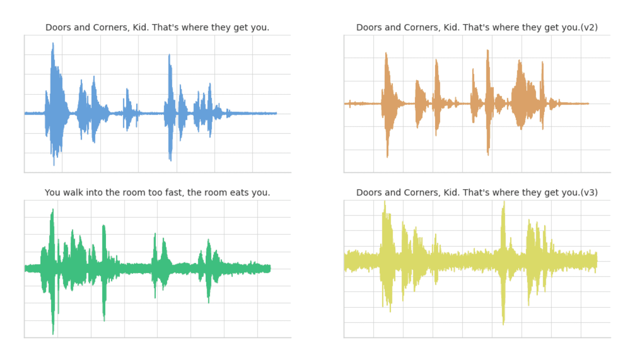
Below are visualizations using matplotlib of the four audio clips:
- Clip 1: This is our base time series based on the quote "Doors and corners, kid. That's where they get you".
- Clip 2: This is a new time series [v2] based on clip 1 where the intonation and speech pattern is extremely exaggerated.
- Clip 3: This is another time series that's based on the quote "You walk into a room too fast, the room eats you." with the same intonation and speed as Clip 1.
- Clip 4: This is a new time series [v3] based on clip 1 where the intonation and speech pattern is similar to clip 1.
The code to read these audio clips and visualize them using matplotlib can be summarized in the following code snippet.
from scipy.io import wavfile from matplotlib import pyplot as plt from matplotlib.pyplot import figure # Read stored audio files for comparison fs, data = wavfile.read("/dbfs/folder/clip1.wav") # Set plot style plt.style.use('seaborn-whitegrid') # Create subplots ax = plt.subplot(2, 2, 1) ax.plot(data1, color='#67A0DA') ... # Display created figure fig=plt.show() display(fig)
The full code-base can be found in the notebook Dynamic Time Warping Background.
As noted below, when the two clips (in this case, clips 1 and 4) have different intonations (amplitude) and latencies for the same quote.
If we were to follow a traditional Euclidean matching (per the following graph), even if we were to discount the amplitudes, the timings between the original clip (blue) and the new clip (yellow) do not match.
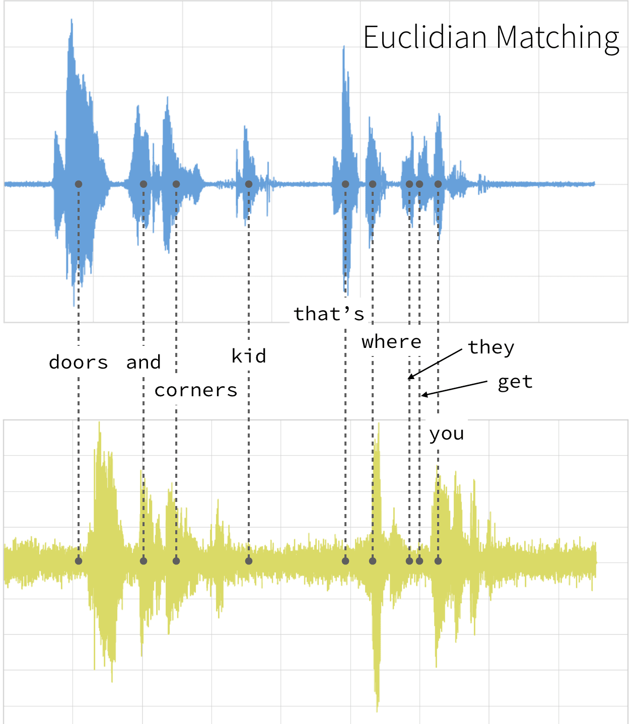
With dynamic time warping, we can shift time to allow for a time series comparison between these two clips.
For our time series comparison, we will use the [fastdtw](https://pypi.org/project/fastdtw/) PyPi library; the instructions to install PyPi libraries within your Databricks workspace can be found here: Azure | AWS. By using fastdtw, we can quickly calculate the distance between the different time series.
from fastdtw import fastdtw # Distance between clip 1 and clip 2 distance = fastdtw(data_clip1, data_clip2)[0] print("The distance between the two clips is %s" % distance)
The full code-base can be found in the notebook Dynamic Time Warping Background.
| Base | Query | Distance |
|---|---|---|
| Clip 1 | Clip 2 | 480148446.0 |
| Clip 3 | 310038909.0 | |
| Clip 4 | 293547478.0 |
Some quick observations:
- As noted in the preceding graph, Clips 1 and 4 have the shortest distance as the audio clips have the same words and intonations
- The distance between Clips 1 and 3 is also quite short (though longer than when compared to Clip 4) even though they have different words, they are using the same intonation and speed.
- Clips 1 and 2 have the longest distance due to the extremely exaggerated intonation and speed even though they are using the same quote.
As you can see, with dynamic time warping, one can ascertain the similarity of two different time series.
The phrase "dynamic time warping," at first read, might evoke images of Marty McFly driving his DeLorean at 88 MPH in the Back to the Future series. Alas, dynamic time warping does not involve time travel; instead, it's a technique used to dynamically compare time series data when the time indices between comparison data points do not sync up perfectly.
As we'll explore below, one of the most salient uses of dynamic time warping is in speech recognition -- determining whether one phrase matches another, even if it the phrase is spoken faster or slower than its comparison. You can imagine that this comes in handy to identify the "wake words" used to activate your Google Home or Amazon Alexa device -- even if your speech is slow because you haven't yet had your daily cup(s) of coffee.
Dynamic time warping is a useful, powerful technique that can be applied across many different domains. Once you understand the concept of dynamic time warping, it's easy to see examples of its applications in daily life, and its exciting future applications. Consider the following uses:
- Financial markets -- comparing stock trading data over similar time frames, even if they do not match up perfectly. For example, comparing monthly trading data for February (28 days) and March (31 days).
- Wearable fitness trackers -- more accurately calculating a walker's speed and the number of steps, even if their speed varied over time.
- Route calculation -- calculating more accurate information about a driver's ETA, if we know something about their driving habits (for example, they drive quickly on straightaways but take more time than average to make left turns).
Data scientists, data analysts, and anyone working with time series data should become familiar with this technique, given that perfectly aligned time-series comparison data can be as rare to see in the wild as perfectly "tidy" data.
In this blog series, we will explore:
- The basic principles of dynamic time warping
- Running dynamic time warping on sample audio data
- Running dynamic time warping on sample sales data using MLflow
The objective of time series comparison methods is to produce a distance metric between two input time series. The similarity or dissimilarity of two-time series is typically calculated by converting the data into vectors and calculating the Euclidean distance between those points in vector space.
Dynamic time warping is a seminal time series comparison technique that has been used for speech and word recognition since the 1970s with sound waves as the source; an often cited paper is Dynamic time warping for isolated word recognition based on ordered graph searching techniques.
This technique can be used not only for pattern matching, but also anomaly detection (e.g. overlap time series between two disjoint time periods to understand if the shape has changed significantly, or to examine outliers). For example, when looking at the red and blue lines in the following graph, note the traditional time series matching (i.e. Euclidean Matching) is extremely restrictive. On the other hand, dynamic time warping allows the two curves to match up evenly even though the X-axes (i.e. time) are not necessarily in sync. Another way is to think of this is as a robust dissimilarity score where a lower number means the series is more similar.
Source: Wiki Commons: File:Euclidean_vs_DTW.jpg
Two-time series (the base time series and new time series) are considered similar when it is possible to map with function f(x) according to the following rules so as to match the magnitudes using an optimal (warping) path.
Traditionally, dynamic time warping is applied to audio clips to determine the similarity of those clips. For our example, we will use four different audio clips based on two different quotes from a TV show called The Expanse. There are four audio clips (you can listen to them below but this is not necessary) -- three of them (clips 1, 2, and 4) are based on the quote:
"Doors and corners, kid. That's where they get you."
and one clip (clip 3) is the quote
"You walk into a room too fast, the room eats you."
|
Doors and Corners, Kid.
That's where they get you. [v1]
|
Doors and Corners, Kid.
That's where they get you. [v2]
|
|
You walk into a room too fast,
the room eats you.
|
Doors and Corners, Kid.
That's where they get you [v3]
|
Quotes are from The Expanse
Below are visualizations using matplotlib of the four audio clips:
- Clip 1: This is our base time series based on the quote "Doors and corners, kid. That's where they get you".
- Clip 2: This is a new time series [v2] based on clip 1 where the intonation and speech pattern is extremely exaggerated.
- Clip 3: This is another time series that's based on the quote "You walk into a room too fast, the room eats you." with the same intonation and speed as Clip 1.
- Clip 4: This is a new time series [v3] based on clip 1 where the intonation and speech pattern is similar to clip 1.
The code to read these audio clips and visualize them using matplotlib can be summarized in the following code snippet.
from scipy.io import wavfile from matplotlib import pyplot as plt from matplotlib.pyplot import figure # Read stored audio files for comparison fs, data = wavfile.read("/dbfs/folder/clip1.wav") # Set plot style plt.style.use('seaborn-whitegrid') # Create subplots ax = plt.subplot(2, 2, 1) ax.plot(data1, color='#67A0DA') ... # Display created figure fig=plt.show() display(fig)
The full code-base can be found in the notebook Dynamic Time Warping Background.
As noted below, when the two clips (in this case, clips 1 and 4) have different intonations (amplitude) and latencies for the same quote.
If we were to follow a traditional Euclidean matching (per the following graph), even if we were to discount the amplitudes, the timings between the original clip (blue) and the new clip (yellow) do not match.
With dynamic time warping, we can shift time to allow for a time series comparison between these two clips.
For our time series comparison, we will use the [fastdtw](https://pypi.org/project/fastdtw/) PyPi library; the instructions to install PyPi libraries within your Databricks workspace can be found here: Azure | AWS. By using fastdtw, we can quickly calculate the distance between the different time series.
from fastdtw import fastdtw # Distance between clip 1 and clip 2 distance = fastdtw(data_clip1, data_clip2)[0] print("The distance between the two clips is %s" % distance)
The full code-base can be found in the notebook Dynamic Time Warping Background.
| Base | Query | Distance |
|---|---|---|
| Clip 1 | Clip 2 | 480148446.0 |
| Clip 3 | 310038909.0 | |
| Clip 4 | 293547478.0 |
Some quick observations:
- As noted in the preceding graph, Clips 1 and 4 have the shortest distance as the audio clips have the same words and intonations
- The distance between Clips 1 and 3 is also quite short (though longer than when compared to Clip 4) even though they have different words, they are using the same intonation and speed.
- Clips 1 and 2 have the longest distance due to the extremely exaggerated intonation and speed even though they are using the same quote.
As you can see, with dynamic time warping, one can ascertain the similarity of two different time series.
ACCURATE REAL-TIME WINDOWED TIME WARPING Robert Macrae Centre for Digital Music Queen Mary University of London [email protected] Simon Dixon Centre for Digital Music Queen Mary University of London [email protected] ABSTRACT Dynamic Time Warping (DTW) is used to find alignments between two related streams of information and can be used to link data, recognise patterns or find similarities. Typically, DTW requires the complete series of both input streams in advance and has quadratic time and space requirements. As such DTW is unsuitable for real-time applications and is inefficient for aligning long sequences. We present Windowed Time Warping (WTW), a variation on DTW that, by dividing the path into a series of DTW windows and making use of path cost estimation, achieves alignments with an accuracy and efficiency superior to other leading modifications and with the capability of synchronising in real-time. We demonstrate this method in a score following application. Evaluation of the WTW score following system found 97.0% of audio note onsets were correctly aligned within 2000 ms of the known time. Results also show reductions in execution times over state-of-theart efficient DTW modifications. 1. INTRODUCTION Dynamic Time Warping (DTW) is used to synchronise two related streams of information by finding the lowest cost path linking feature sequences of the two streams together. It has been used for audio synchronisation [3], cover song identification [13], automatic transcription [14], speech processing [10], gesture recognition [7], face recognition [1], lip-reading [8], data-mining [5], medicine [15], analytical chemistry [2], and genetics [6], as well as other areas. In DTW, dynamic programming is used to find the minimal cost path through an accumulated cost matrix of the elements of two sequences. As each element from one sequence has to be compared with each element from the other, the calculation of the matrix scales inefficiently with longer sequences. This, combined with the requirement of knowing the start and end points of the sequences, makes DTW unsuitable for real-time synchronisation. A real-time variant would make DTW viable at larger scales and capable of driving applications such as score following, automatic accompaniment and live gesture recognition. Permission to make digital or hard copies of all or part of this work for personal or classroom use is granted without fee provided that copies are not made or distributed for profit or commercial advantage and that copies bear this notice and the full citation on the first page. c 2010 International Society for Music Information Retrieval. Local constraints such as those by Sakoe and Chiba [10] improve the efficiency of DTW to linear time and space complexity by limiting the potential area of the accumulated cost matrix to within a set distance of the diagonal. However, not all alignments necessarily fit within these bounds. Salvador and Chan proposed, in FastDTW [11], a multi-resolution DTW where increasingly higher resolution DTW paths are bounded by a band around the previous lower resolution path, leading to large reductions in the execution time. On-Line Time Warping by Dixon [3] made real-time synchronisation with DTW possible by calculating the accumulated cost in a forward manner and bounding the path by a forward path estimation. While the efficiency of DTW has been addressed in FastDTW [11] and the real-time aspect has been made possible with On-Line Time Warping [3], WTW contributes to synchronisation by offering steps to further improve the efficiency whilst working in a progressive (real-time applicable) manner and preserving the accuracy of standard DTW. This method consists of breaking down the alignment into a series of separate bounded sub-paths and using a cost estimation to limit the area of the accumulated cost matrix calculated to small regions covering the alignment. In Section 2 we explain conventional DTW before describing how WTW works in Section 3. In Section 4 we evaluate the accuracy and efficiency of WTW in a score following application. Finally, in Section 5, we draw conclusions from this work and discuss future improvements. 2. DYNAMIC TIME WARPING DTW requires two sets of features to be extracted from the two input pieces being aligned and a function for calculating the similarity between any two frames of these feature sets. One such measurement of the similarity is the inner product. As the inner product returns a high value for similar frames, we subtract the inner product from one so that the optimal path cost is the path with the minimal cost. Equation 1 shows how to calculate this similarity measurement between frames Am and Bn from feature sequences A = (a1, a2, ..., aM) and B = (b1, b2, ..., bN ) respectively: dA,B(m, n) = 1 - < am, bn > kamkkbnk (1) Dynamic programming is used to find the optimum path, P = (p1, p2, ..., pW ), through the similarity matrix C(m, n) 423 11th International Society for Music Information Retrieval Conference (ISMIR 2010) Figure 1. Dynamic Time Warping aligning audio with a musical score. The audio is divided into chroma frames (bottom) which are then compared against the score's chroma frames (left). The similarity matrix (centre) shows a path where the sequences have the lowest cost (highest similarity). Any point on this path indicates where in the score the corresponding audio relates to. with m ∈ [1 : M] and n ∈ [1 : N] where each pk = (mk, nk) indicates that frames amk and bnk are part of the aligned path at position k. An example of this similarity matrix, including the features used and the lowest cost path, can be seen in Figure 1. The final path is guaranteed to have the minimal overall cost D(P) = PW k=1 dA,B(mk, nk), within the limits of the features used, whilst satisfying the following conditions: Bounds: p1 = (1, 1) pW = (M, N) Monotonicity: mk+1 ≥ mk for all k ∈ [1, W - 1] nk+1 ≥ nk for all k ∈ [1, W - 1] Continuity: mk+1 ≤ mk + 1 for all k ∈ [1, W - 1] nk+1 ≤ nk + 1 for all k ∈ [1, W - 1] 3. WINDOWED TIME WARPING WTW consists of calculating small sub-alignments and combining these to form an overall path. Subsequent sub-paths are started from points along the previous sub-paths. Realtime path positions can then be extrapolated from these sub-paths. The end points of these sub-alignments are either undirected, by assuming they lie on the diagonal, or directed, by using a forward path estimate. As such WTW can be seen as a two-pass system similar to FastDTW and OTW. The sub-alignments make use of an optimisation that avoids calculating points with costs that are over the cost estimate (provided by the initial direction path), referred to as the A-Star Cost Matrix. WTW also requires the use of Features, Window Dimensions, and Local Constraints that all affect how the alignments are made. The overall process is outlined in Algorithm 1. In order to demonstrate WTW we implemented a score following application using this method to synchronise audio and musical scores. Input: Feature Sequence A and Feature Sequence B Output: Alignment Path Path = new Path.starting(1,1); while Path.length < min (A.length,B.length) do Start = Path.end; End = Start; while (End - Start).length < Window Size do End = argmin(Inner Product(End.next points)); end Cost Estimate = End.cost; A-Star Matrix = A Star Fill Rect(Start,End,Cost Estimate); Path.add(A Star Matrix.getPath(1,Hop Size)); end return Path; Algorithm 1: The Windowed Time Warping algorithm. 3.1 Features The feature vector describes how the sequence data is represented and segmented. The sequence is divided up into feature frames in order to differentiate the changes in the sequence over time. The frame size and spacing are referred to as the window size and hop size respectively. The implementation of WTW for score following requires a musically based feature vector. In this case, we use chroma features, a 12 dimensional vector corresponding to the unique pitch classes in standard Western music. The intensities of the chroma vectors can be seen as a representation of the harmonic and melodic content of the music. In our implementation we use a window size of 200ms and a hop size of 50ms. 3.2 Window Dimensions Similar to how the sequence data is segmented, the windows of standard DTW in WTW have a window size and hop size to describe their size and spacing respectively. A larger window size and/or smaller hop size will increase the accuracy of the alignment, as more of the cost matrix is calculated, however will this will be less efficient. Examples of different window and hop sizes can be seen in Figure 2 and a comparison of Window and Hop sizes is made in Section 4. 3.3 Local Constraints We refer to two types of local constraints in Dynamic Programming. The first, henceforth known as the cost constraint, indicates the possible predecessors of a point pk on a path. The predecessor pk-1 with lowest path cost D(pk-1) is chosen when calculating the accumulated cost 424 11th International Society for Music Information Retrieval Conference (ISMIR 2010) Figure 2. The regions of the similarity matrix computed for various values of the window size (top row) and hop size (bottom row). Figure 3. Some example local constraints as defined by Rabiner and Juang [9]. matrix. The second, referred to as the movement constraint, indicates the possible successors of a point pk. Standard DTW doesn't make use of a movement constraint as all the frames in the cost matrix are calculated. Examples of local constraints by Rabiner and Juang [9] are show in Figure 3. These constraints define the characteristics of the dynamic programming. For example, Type I allows for horizontal and vertical movement which corresponds to a single frame of one sequence being linked to multiple frames of the other. All the other Types allow high cost frames to be skipped and Type III and II show how the paths can skip these frames directly or add in the single steps, respectively. The two path finding algorithms, described next, make use of the Type I and a modified version of the Type VII (where the steps are taken directly as in Type III) local constraints. 3.4 Window Guidance The sequential windows that make up the alignment of WTW can be either directed or undirected. Whilst it can help to direct the end point of the windows of DTW (particularly for alignments between disproportional sequences where the expected path angle will be far from 45◦ ), the sub-paths calculated within these windows can make up for an error in the estimation. A low hop size should ensure the point taken from the sub-path as the starting point for the next window is likely to be on the correct path. For the windows to be directed, a forward estimation is required. The Forward Greedy Path (FGP) is an algorithm which makes steps through the similarity matrix based on whichever subsequent step has the highest similarity (minimal cost) using a movement constraint to decide which frames are considered. In this manner the path can work in an efficient forward progressive manner, however, will be more likely to be thrown off the correct path by any periods of dissimilarity within the alignment. The first FGP path F = (f1, f2, ..., fW ) where fk = (mk, nk) starts from position f1 = (m1, n1) and from then on each subsequent frame is determined by whichever of the available frames, as determined by the local constraint, has the lowest cost. Therefore the total cost D(m, n) to any point (m, n) on the FGP path F is D(fk) = Pk l=1 d(fl) and any point is dependent on the previous point: fk+1 = argmin(d(i, j)) where the range of possible values for i and j are determined by fk and the local constraints. The FGP path only needs to calculate similarities between frames considered within the local constraints and so at this stage a vast majority of the similarity matrix does not need to be calculated. When the FGP reaches fW , the window size, the final point fW = (mW , nW ) is selected as the end point for the accumulated cost-matrix. Note that some combinations of constraints that skip points (i.e. where i or j are greater than 1) will require that jumps in the FGP are filled in order to compute a complete cost estimate, like in the Type V local constraint, so that the cost estimation of the FGP is complete. A comparison of guidance measures is made in Section 4. 3.5 A-Star Cost Matrix The windowed area selected is calculated as an accumulated cost matrix between the beginning and end points of the FGP i.e. C(m, n) of m ∈ [mf1 : mfL ] and n ∈ [nf1 : nfL ]. This accumulated cost matrix can be calculated in either a forward or reverse manner, linking the start to the end point or vice versa. This uses the standard Type I cost constraint to determine a frame's accumulated cost as shown by Equation 2: D(m, n) = d(m, n) + min D(m - 1, n - 1) D(m - 1, n) D(m, n - 1) (2) The sub-path S = (s1, s2, ..., sV ) is given by the accumulated cost constraints by following the cost progression from the beginning point in this window until the hop size is reached. When the sub-path reaches sV , the final point fV = (mv, nv) is then taken as the starting point for the next window and so on until the end of either sequence is reached. The sub-paths are concatenated to construct the global WTW path. This process can also be seen in Figure 4. Either of the undirected and directed window end point estimations provide an estimate cost D(F) for each subpath. This estimate can be used to disregard any points within the accumulated cost matrix that are above this cost 425 11th International Society for Music Information Retrieval Conference (ISMIR 2010) Figure 4. The complete Windowed Time Warping path. as it is known there is a potential sub-path that is cheaper. The calculation of the similarity for most of these inefficient points can be avoided by calculating the accumulated cost matrix in rows and columns from the end point fL to the start f1. When each possible preceding point for the next step of the current row/column has a total cost above the estimated cost i.e. min(D(m-1, n-1), D(m- 1, n), D(m, n - 1)) >= D(F) the rest of the row/column is then set as more than the cost estimate, thus avoiding calculating the accumulated cost for a portion of the matrix. This procedure can be seen in Figure 5. 4. EXPERIMENTAL EVALUATION To evaluate WTW we used the score following system with ground truth MIDI, audio and path reference files and compared the accuracy of the found alignments with the known alignments. MATCH, the implementation of On-Line Time Warping [4], was also used to align the test pieces for comparison purposes. In both cases the MIDI was converted to audio using Timidity. 4.1 Mazurka Test Data The CHARM Mazurka Project by the Centre for the History and Analysis of Recorded Music led by Nick Cook at Royal Holloway, University of London has published a large number of linked metadata files for Mazurka recordings in the form of reverse conducted data, 1 produced by Craig Sapp [12]. We then used template matching to combine this data with MIDI files, establishing links between MIDI notes and reverse conducted notes at the ms level. This provided a set of ground truth files linking the MIDI score to the audio recordings. These ground truths were compared with an off-line DTW alignment and manually supervised to correct any differences found. Overall, 217 1 http://mazurka.org.uk/info/revcond/ Figure 5. The calculation of the accumulated cost matrix. The numbering shows the order in which rows and columns are calculated and the progression of the path finding algorithm is shown by arrows. Dark squares represent a total cost greater than the estimated path cost whilst black squares indicate points in the accumulated cost matrix that do not need to be calculated. sets of audio recordings, MIDI scores and reference files were produced. 4.2 Evaluation Metrics For each path produced by WTW, each estimated audio note time was compared with the reference and the difference was recorded. For differing levels of accuracy requirements (100 ms, 200 ms, 500 ms and 2000 ms), the percentages of notes that were estimated correctly within this requirement for each piece were recorded. These piecewise accuracies are then averaged for an overall rating. The 2000 ms accuracy requirement is used as the MIREX score following accuracy requirement for notes hit. 4.3 Window Dimensions The effect of the window size and hop size in WTW is examined in Table 1. The accuracy tests (shown in the top half) show a trend that suggests larger window sizes and smaller hop sizes lead to greater accuracy, as is similar to feature frame dimensions. However, larger window sizes and smaller hop sizes also lead to slower execution times as more points on the similarity matrix were calculated. 4.4 Window Guidance A comparison of guidance methods for WTW is shown in Table 2. This comparison shows that for the test data used, there was not much difference between directed and undirected WTW and directed only offered an improvement when a large local constraint was used. 426 11th International Society for Music Information Retrieval Conference (ISMIR 2010) Alignment Accuracy at 2000 ms Window Size Hop Size 100 200 300 400 100 76.0% 83.1% 81.8% 81.9% 200 63.7% 82.2% 82.0% 82.0% 300 57.7% 77.7% 81.2% 82.5% 400 57.4% 66.1% 81.1% 82.0% Table 1. Accuracy test results comparing different window and hop sizes for WTW. For this test there was a guidance FGP that used a Type VII +6 movement constraint (see Table 2) and the accumulated cost matrix used a Type I cost constraint and Type I movement constraint. Alignment Accuracy Acc. Req. 100 ms 200 ms 500 ms 2000 ms None 63.8% 75.9% 82.0% 86.9% Type I 56.2% 68.7% 74.2% 78.1% Type IV 63.3% 74.8% 80.7% 86.0% Type VII 64.0% 76.9% 82.6% 86.6% Type IV +4 58.0% 70.3% 75.8% 79.5% Type VII +6 59.4% 72.2% 78.0% 81.2% Type II 63.9% 75.8% 81.8% 87.3% Type V 64.9% 78.0% 83.9% 88.1% Table 2. Accuracy test results comparing different methods for guiding the windows in WTW. The name of the guidance method refers to the movement constraint used in the Forward Greedy Path. The 'Type 4 +4' and 'Type 7 +6' constraints include additional horizontal and vertical frames to complete the block. For this test the window and hop size were set at 300ms and the accumulated cost matrix used a Type I cost constraint and Type I movement constraint. 4.5 Accuracy Results The results of the accuracy test can be seen in Table 3. From this test we can see WTW produces an accuracy rate comparable with that of OTW. What separates the two methods is that the OTW method took on average 7.38 seconds to align a Mazurka audio and score file where as WTW took 0.09 seconds, (approximately one 80th of the time of OTW). The average length of the Mazurka recordings is 141.3 seconds, therefore, in addition to having the ability to calculate the alignment path sequentially, both methods achieve greater than real-time performance by some margin. 4.6 Efficiency Results The efficiency tests consisted of aligning sequences of different lengths and recording the execution time. The results of this test can be seen in Table 4. These results show that WTW has linear time costs in relation to the length of the input sequence, unlike standard DTW. The optimisations suggested in this work are shown to decrease the time cost in aligning larger sequences over FastDTW. Alignment Accuracy Acc. Req. 100 ms 200 ms 500 ms 2000 ms WTW 73.6% 88.8% 94.9% 97.0% OTW 70.9% 86.7% 94.8% 97.3% Table 3. Accuracy test results comparing WTW and OTW estimated audio note onset times against references for 217 Mazurka recordings at 4 levels of accuracy requirements. For this test the window and hop size were set at 300ms and the accumulated cost matrix used a Type I cost constraint and Type VII movement constraint. Execution time (seconds) Sequence length 100 1000 10000 100000 DTW 0.02 0.92 57.45 7969.59 FastDTW (r100) 0.02 0.06 8.42 207.19 WTW 0.002 0.06 0.90 9.52 Table 4. Efficiency test results showing the execution time (in seconds) for 4 different lengths of input sequences (in frames). Results for FastDTW and DTW are from [11]. The r value for FastDTW relates to the radius factor. 5. DISCUSSION AND CONCLUSION This paper has introduced WTW, a linear cost variation on DTW for real-time synchronisations. WTW breaks down the regular task of creating an accumulated cost matrix between the complete series of input sequence vectors, into small, sequential, cost matrices. Additional optimisations include local constraints in the dynamic programming and cut-off limits for the accumulated cost matrices. Evaluation of WTW has shown it to be more efficient than state of the art DTW based off-line alignment techniques. WTW has also been shown to match the accuracy of OTW whilst improving on the time taken to process files. Whilst this difference has little effect when synchronising live sequences on standard computers, the greater efficiency of WTW could be useful in running real-time synchronisation methods on less powerful processors, such as those in mobile phones, or when data-mining large datasets for tasks such as cover song identification. Future work will involve evaluating WTW on a wider variety of test data-sets, including non-audio related tasks and features. Possible improvements may be found in novel local constraints and/or the dynamic programming used to estimate the start and end points of the accumulated cost matrices. Presently, WTW assumes the alignment is continuous from the start to the end. A more flexible approach will be required to handle alignments made of partial sequence matches. Also, the modifications of WTW could potentially be combined with other modifications of DTW, such as those in FastDTW in order to pool efficiencies. Lastly, WTW, like DTW, is applicable to a number of tasks that involve data-mining, recognition systems or similarity measures. It is hoped WTW makes DTW viable for applications on large data sets in a wide range of fields. 427 11th International Society for Music Information Retrieval Conference (ISMIR 2010) 6. ACKNOWLEDGMENTS This work is supported by the EPSRC project OMRAS2 (EP/ E017614/1). Robert Macrae is supported by an EPSRC DTA Grant. 7. REFERENCES [1] Bir Bhanu and Xiaoli Zhou. Face recognition from face profile using dynamic time warping. In ICPR '04: Proceedings of the Pattern Recognition, 17th International Conference on (ICPR'04) Volume 4, pages 499--502, Washington, DC, USA, 2004. IEEE Computer Society. [2] David Clifford, Glenn Stone, Ivan Montoliu, Serge Rezzi, Franc¸ois-Pierre Martin, Philippe Guy, Stephen Bruce, and Sunil Kochhar. Alignment using variable penalty dynamic time warping. Analytical Chemistry, 81(3):1000--1007, January 2009. [3] Simon Dixon. Live tracking of musical performances using on-line time warping. In Proceedings of the 8th International Conference on Digital Audio Effects, pages 92--97, Madrid, Spain, 2005. [4] Simon Dixon and Gerhard Widmer. MATCH: A music alignment tool chest. In Proceedings of the 6th International Conference on Music Information Retrieval, page 6, 2005. [5] Eamonn J. Keogh and Michael J. Pazzani. Scaling up dynamic time warping for datamining applications. In Proceedings of the sixth ACM SIGKDD international conference on Knowledge discovery and data mining, pages 285--289, New York, NY, USA, 2000. ACM. [6] Beno'ıt Legrand, C. S. Chang, S. H. Ong, Soek-Ying Neo, and Nallasivam Palanisamy. Chromosome classification using dynamic time warping. Pattern Recogn. Lett., 29(3):215--222, 2008. [7] Meinard Muller. ¨ Information Retrieval for Music and Motion. Springer-Verlag New York, Inc., Secaucus, NJ, USA, 2007. [8] Hiroshi Murase and Rie Sakai. Moving object recognition in eigenspace representation: gait analysis and lip reading. Pattern Recogn. Lett., 17(2):155--162, 1996. [9] Lawrence Rabiner and Biing-Hwang Juang. Fundamentals of speech recognition. Prentice-Hall, Inc., Upper Saddle River, NJ, USA, 1993. [10] Hiroaki Sakoe and Seibi Chiba. Dynamic programming algorithm optimization for spoken word recognition. IEEE Transactions on Acoustics, Speech, and Signal Processing, 26(1), 1978. [11] Stan Salvador and Philip Chan. FastDTW: Toward accurate dynamic time warping in linear time and space. In Workshop on Mining Temporal and Sequential Data, page 11, 2004. [12] Craig Sapp. Comparative analysis of multiple musical performances. In Proceedings of the International Conference on Music Information Retrieval (ISMIR) 2007, pages 497--500, 2007. [13] J Serra, E G ` omez, P Herrera, and X Serra. Chroma ' binary similarity and local alignment applied to cover song identification. Audio, Speech, and Language Processing, IEEE Transactions on, 16(6):1138--1151, 2008. [14] Robert J. Turetsky and Daniel P.W. Ellis. Ground-truth transcriptions of real music from force-aligned midi syntheses. In Proceedings of the 4th International Conference on Music Information Retrieval, 2003. [15] H. J. L. M. Vullings, M. H. G. Verhaegen, and H. B. Verbruggen. Automated ECG segmentation with dynamic time warping. In Proceedings of the 20th Annual International Conference of the IEEE In Engineering in Medicine and Biology Society, 1998, volume 1, pages 163--166, 1998. 428 11th International Society for Music Information Retrieval Conference (ISMIR 2010)
Image the following situation: You inspect a delivery of new time series data and want to develop a classification algorithm for it. Because it is a new dataset for you, you are not sure if you should use a shape based approach or maybe a feature based one. In any case, you want to apply different packages on that data and compare the results.
Now, there is no widely agreed standard for time series data. For most of the tools,
- you will have to read the instructions
- understand the format of the respective package,
- and finally you will have write a script to convert your data.
This is annoying and slows you down.
For the construction of supervised machine learning models, using different packages is way more convenient.
Almost all packages expect a feature matrix as input.
In a feature matrix, a column denotes a feature, a row is a sample.
Object wise, either numpy.ndarrays or their extensions pandas.DataFrame are used.
You can use your feature matrix and first apply models from sklearn on it. Then you can take the same object and try lightgbm or xgboost models on it:
X = [[0, 0, 1, 1],
     [0, 1, 0, 0],
     [1, 0, 0, 1]]

y = [1,
     1,
     1]

# first train a model from sklearn
from sklearn.ensemble import RandomForestClassifer()
clf1 = RandomForestClassifer()
clf1.fit(X, y)

# now train a model from another package on the data, there is no transformation necessary
from lightgbm import LGBMClassifier
clf2 = LGBMClassifier()
clf2.fit(X, y)
All without every having the need to convert your data, everything works out of the box.
We want the same for time series data. The purpose of this document is to find a common standard. The analysis of time series data and the interplay between packages should become more user friendly.
A time series consists of timely annotated data, a recording is based on two characteristics, the time and value dimensions.
Therefore, a singular recording is a two dimensional vector
(time, value)
An example would be
(2009-06-15T13:45:30, 83°C)
which denotes a temperature of 83°C measured at time 2009-06-15T13:45:30.
A whole time series, which is a collection of such two dimensional recordings can have meta information, characteristics that will not change over time. The most important meta information is the identifier of the respective entity and in case of multivariate scenarios the type of time series. Multivariate means that a singular entity has multiple assigned time series.
In that case, a recording is a 4 dimensional vector
(id, time, value, kind)
where value is the value of the time series of type kind recorded at time time for the entity id.
For example
(VW Beetle - SN: 7 4545 4543, 2009-06-15T13:45:30, 83°C, Engine Temperature G1)
denotes a temperature of 83°C measured at sensor Engine Temperature G1 for the VW Beetle with serial number 7 4545 4543 at time 2009-06-15T13:45:30.
There is a myriad of different formats which could be used to save such information. We will discuss the following formats.
- Relational
- Stacked matrix
- Flat matrix
- 3-dimensional matrix
- Nested
- Dictionary based
- Binary
- ?
(If you have some more ideas, please feel free to submit a pr). Later we will analyze the saving capabilities of the different formats.
This is the most flexible format. It supports non uniformly sampled time series of different lengths. In this format, each row will contain the four dimensional tuple.
Example: The two time series
values [11, 2] for times [0, 1] of kind a for id 1
values [13, 4] for times [0, 3] of kind b for id 1
will be saved as
time  id  value kind
0     1    11    a
1     1     2    a
0     1    13    b
3     1     4    b
Is suitable for the multivariate, uniformly sampled case when we want to save different kinds of time series that all need to have the same length and need to be recorded at the same times.
In this format, we will dedicate a full columns for each type of time series.
Example: The two time series
values [11, 2] for times [0, 1] of kind a for id 1
values [13, 4] for times [0, 1] of kind b for id 1
will be saved as
time  id  a   b
0     1  11  13
1     1   2   4
For this format, the time series need to be uniformly sampled and of same length. Then we use the first two dimensions of the matrix to denote kind and id and the third one for the time scale.
Example: The two time series
values [11, 2] for times [0, 1] of kind a for id 1
values [13, 4] for times [0, 1] of kind b for id 1
will be recorded as
    time         a        b
1   [0, 1]  [11, 2]  [13, 4]
We can have dictionary mapping from the id to another dictionary that maps kind to the time series. Essentially you are using a singular array for each time series.
Example: The two time series
values [11, 2] for times [0, 1] of kind a for id 1
values [13, 4] for times [0, 3] of kind b for id 1
will be recorded as
{ 1:
  { a: [time: [0, 1], value:[11, 2]],
    b: [time: [0, 3], value:[13, 4]]
  }
}
Before one can pick the right format, one needs to check a few points
- Do the time series can have different lengths?
- Are the time series non uniformly sampled, are the time series allowed to have missing values?
- Do we inspect multivariate time series?
Depending of the answers to this questions, different formats are suitable. The following table lists the characteristics of the different formats
| Format | 1. Different length | 2. Non uniformly sampled | 3. Multivariate time series | Does not contain redundant information | Tabular format |
|---|---|---|---|---|---|
| 1.i Stacked Matrix | X | X | X | X | |
| 1.ii Flat Matrix | X | X | X | ||
| 1.iii 3-dimensional Matrix | X | X | |||
| 2.ii Dictionary based | X | X | X | X |
Dynamic Time Warping(DTW) is an algorithm for measuring similarity between two temporal sequences which may vary in speed. For instance, similarities in walking could be detected using DTW, even if one person was walking faster than the other, or if there were accelerations and decelerations during the course of an observation. It can be used to match a sample voice command with others command, even if the person talks faster or slower than the prerecorded sample voice. DTW can be applied to temporal sequences of video, audio and graphics data-indeed, any data which can be turned into a linear sequence can be analyzed with DTW.
In general, DTW is a method that calculates an optimal match between two given sequences with certain restrictions. But let's stick to the simpler points here. Let's say, we have two voice sequences Sample and Test, and we want to check if these two sequences match or not. Here voice sequence refers to the converted digital signal of your voice. It might be the amplitude or frequency of your voice that denotes the words you say. Let's assume:
Sample = {1, 2, 3, 5, 5, 5, 6}
Test   = {1, 1, 2, 2, 3, 5}
We want to find out the optimal match between these two sequences.
At first, we define the distance between two points, d(x, y) where x and y represent the two points. Let,
d(x, y) = |x - y| //absolute difference
Let's create a 2D matrix Table using these two sequences. We'll calculate the distances between each point of Sample with every points of Test and find the optimal match between them.
+------+------+------+------+------+------+------+------+
|      |   0  |   1  |   1  |   2  |   2  |   3  |   5  |
+------+------+------+------+------+------+------+------+
|   0  |      |      |      |      |      |      |      |
+------+------+------+------+------+------+------+------+
|   1  |      |      |      |      |      |      |      |
+------+------+------+------+------+------+------+------+
|   2  |      |      |      |      |      |      |      |
+------+------+------+------+------+------+------+------+
|   3  |      |      |      |      |      |      |      |
+------+------+------+------+------+------+------+------+
|   5  |      |      |      |      |      |      |      |
+------+------+------+------+------+------+------+------+
|   5  |      |      |      |      |      |      |      |
+------+------+------+------+------+------+------+------+
|   5  |      |      |      |      |      |      |      |
+------+------+------+------+------+------+------+------+
|   6  |      |      |      |      |      |      |      |
+------+------+------+------+------+------+------+------+
Here, Table[i][j] represents the optimal distance between two sequences if we consider the sequence up to Sample[i] and Test[j], considering all the optimal distances we observed before.
For the first row, if we take no values from Sample, the distance between this and Test will be infinity. So we put infinity on the first row. Same goes for the first column. If we take no values from Test, the distance between this one and Sample will also be infinity. And the distance between 0 and 0 will simply be 0. We get,
+------+------+------+------+------+------+------+------+
|      |   0  |   1  |   1  |   2  |   2  |   3  |   5  |
+------+------+------+------+------+------+------+------+
|   0  |   0  |  inf |  inf |  inf |  inf |  inf |  inf |
+------+------+------+------+------+------+------+------+
|   1  |  inf |      |      |      |      |      |      |
+------+------+------+------+------+------+------+------+
|   2  |  inf |      |      |      |      |      |      |
+------+------+------+------+------+------+------+------+
|   3  |  inf |      |      |      |      |      |      |
+------+------+------+------+------+------+------+------+
|   5  |  inf |      |      |      |      |      |      |
+------+------+------+------+------+------+------+------+
|   5  |  inf |      |      |      |      |      |      |
+------+------+------+------+------+------+------+------+
|   5  |  inf |      |      |      |      |      |      |
+------+------+------+------+------+------+------+------+
|   6  |  inf |      |      |      |      |      |      |
+------+------+------+------+------+------+------+------+
Now for each step, we'll consider the distance between each points in concern and add it with the minimum distance we found so far. This will give us the optimal distance of two sequences up to that position. Our formula will be,
Table[i][j] := d(i, j) + min(Table[i-1][j], Table[i-1][j-1], Table[i][j-1])
For the first one, d(1, 1) = 0, Table[0][0] represents the minimum. So the value of Table[1][1] will be 0 + 0 = 0. For the second one, d(1, 2) = 0. Table[1][1] represents the minimum. The value will be: Table[1][2] = 0 + 0 = 0. If we continue this way, after finishing, the table will look like:
+------+------+------+------+------+------+------+------+
|      |   0  |   1  |   1  |   2  |   2  |   3  |   5  |
+------+------+------+------+------+------+------+------+
|   0  |   0  |  inf |  inf |  inf |  inf |  inf |  inf |
+------+------+------+------+------+------+------+------+
|   1  |  inf |   0  |   0  |   1  |   2  |   4  |   8  |
+------+------+------+------+------+------+------+------+
|   2  |  inf |   1  |   1  |   0  |   0  |   1  |   4  |
+------+------+------+------+------+------+------+------+
|   3  |  inf |   3  |   3  |   1  |   1  |   0  |   2  |
+------+------+------+------+------+------+------+------+
|   5  |  inf |   7  |   7  |   4  |   4  |   2  |   0  |
+------+------+------+------+------+------+------+------+
|   5  |  inf |  11  |  11  |   7  |   7  |   4  |   0  |
+------+------+------+------+------+------+------+------+
|   5  |  inf |  15  |  15  |  10  |  10  |   6  |   0  |
+------+------+------+------+------+------+------+------+
|   6  |  inf |  20  |  20  |  14  |  14  |   9  |   1  |
+------+------+------+------+------+------+------+------+
The value at Table[7][6] represents the maximum distance between these two given sequences. Here 1 represents the maximum distance between Sample and Test is 1.
Now if we backtrack from the last point, all the way back towards the starting (0, 0) point, we get a long line that moves horizontally, vertically and diagonally. Our backtracking procedure will be:
if Table[i-1][j-1] <= Table[i-1][j] and Table[i-1][j-1] <= Table[i][j-1]
    i := i - 1
    j := j - 1
else if Table[i-1][j] <= Table[i-1][j-1] and Table[i-1][j] <= Table[i][j-1]
    i := i - 1
else
    j := j - 1
end if
We'll continue this till we reach (0, 0). Each move has its own meaning:
- A horizontal move represents deletion. That means our Test sequence accelerated during this interval.
- A vertical move represents insertion. That means out Test sequence decelerated during this interval.
- A diagonal move represents match. During this period Test and Sample were same.
Our pseudo-code will be:
Procedure DTW(Sample, Test):
n := Sample.length
m := Test.length
Create Table[n + 1][m + 1]
for i from 1 to n
    Table[i][0] := infinity
end for
for i from 1 to m
    Table[0][i] := infinity
end for
Table[0][0] := 0
for i from 1 to n
    for j from 1 to m
        Table[i][j] := d(Sample[i], Test[j])
                       + minimum(Table[i-1][j-1],      //match
                                 Table[i][j-1],        //insertion
                                 Table[i-1][j])        //deletion
    end for
end for
Return Table[n + 1][m + 1]
We can also add a locality constraint. That is, we require that if Sample[i] is matched with Test[j], then |i - j| is no larger than w, a window parameter.
Complexity:
The complexity of computing DTW is O(m * n) where m and n represent the length of each sequence. Faster techniques for computing DTW include PrunedDTW, SparseDTW and FastDTW.
Applications:
- Spoken word recognition
- Correlation Power Analysis
Find out why DTW is a very useful technique to compare two or more time series signals and add it to your time series analysis toolbox!!
1. Introduction
In this world which is getting dominated by Internet of Things (IoT), there is an increasing need to understand signals from devices installed in households, shopping malls, factories and offices. For example, any voice assistant detects, authenticates and interprets commands from humans even if it is slow or fast. Our voice tone tends to be different during different times of the day. In the early morning after we get up from bed, we interact with a slower, heavier and lazier tone compared to other times of the day. These devices treat the signals as time series and compare the peaks, troughs and slopes by taking into account the varying lags and phases in the signals to come up with a similarity score. One of the most common algorithms used to accomplish this is Dynamic Time Warping (DTW). It is a very robust technique to compare two or more Time Series by ignoring any shifts and speed.
As part of Walmart Real Estate team, I am working on understanding the energy consumption pattern of different assets like refrigeration units, dehumidifiers, lighting, etc. installed in the retail stores.This will help in improving quality of data collected from IoT sensors, detect and prevent faults in the systems and improve energy consumption forecasting and planning. This analysis involves time series of energy consumption during different times of a day i.e. different days of a week, weeks of a month and months of a year. Time series forecasting often gives bad predictions when there is sudden shift in phase of the energy consumption due to unknown factors. For example if the defrost schedule, items refresh routine for a refrigeration unit, or weather changes suddenly and are not captured to explain the phase shifts of energy consumption, it is important to detect these change points.
In the example below, the items refresh routine of a store has shifted by 2 hours on Tuesday leading the shift in peak energy consumption of refrigeration units and this information was not available to us for many such stores.
The peak at 2 am got shifted to 4 am. DTW when run recursively for consecutive days can identify the cases for which phase shift occurred without much change in shape of signals.
The training data can be restricted to Tuesday onwards to improve the prediction of energy consumption in future in this case as phase shift was detected on Tuesday. The setup improved the predictions substantially ( > 50%) for the stores for which the reason of shift was not known. This was not possible by traditional ways of one to one comparison of signals.
In this blog, I will explain how DTW algorithm works and throw some light on the calculation of the similarity score between two time series and its implementation in python. Most of the contents in this blog have been sourced from this paper, also mentioned in the references section below.
2. Why do we need DTW ?
Any two time series can be compared using euclidean distance or other similar distances on a one to one basis on time axis. The amplitude of first time series at time T will be compared with amplitude of second time series at time T. This will result into a very poor comparison and similarity score even if the two time series are very similar in shape but out of phase in time.
DTW compares amplitude of first signal at time T with amplitude of second signal at time T+1 and T-1 or T+2 and T-2. This makes sure it does not give low similarity score for signals with similar shape and different phase.
3. How it works?
Let us take two time series signals P and Q
Series 1 (P) : 1,4,5,10,9,3,2,6,8,4
Series 2 (Q): 1,7,3,4,1,10,5,4,7,4
Step 1 : Empty Cost Matrix Creation
Create an empty cost matrix M with x and y labels as amplitudes of the two series to be compared.
Step 2: Cost Calculation
Fill the cost matrix using the formula mentioned below starting from left and bottom corner.
M(i, j) = |P(i) --- Q(j)| + min ( M(i-1,j-1), M(i, j-1), M(i-1,j) )
where
M is the matrix
i is the iterator for series P
j is the iterator for series Q
Let us take few examples (11,3 and 8 ) to illustrate the calculation as highlighted in the below table.
for 11,
|10 --4| + min( 5, 12, 5 )
= 6 + 5
= 11
Similarly for 3,
|4 --1| + min( 0 )
= 3+ 0
= 3
and for 8,
|1 --3| + min( 6)
= 2 + 6
= 8
The full table will look like this:
Step 3: Warping Path Identification
Identify the warping path starting from top right corner of the matrix and traversing to bottom left. The traversal path is identified based on the neighbour with minimum value.
In our example it starts with 15 and looks for minimum value i.e. 15 among its neighbours 18, 15 and 18.
The next number in the warping traversal path is 14. This process continues till we reach the bottom or the left axis of the table.
The final path will look like this:
Let this warping path series be called as d.
d = [15,15,14,13,11,9,8,8,4,4,3,0]
Step 4: Final Distance Calculation
Time normalised distance , D
where k is the length of the series d.
k = 12 in our case.
D = ( 15 + 15 + 14 + 13 + 11 + 9 + 8 + 8 + 4 + 4 + 3 + 0 ) /12
= 104/12
= 8.63
Let us take another example with two very similar time series with unit time shift difference.
Cost matrix and warping path will look like this.
DTW distance ,D =
( 0 + 0 + 0 + 0 + 0 +0 +0 +0 +0 +0 +0 ) /11
= 0
Zero DTW distance implies that the time series are very similar and that is indeed the case as observed in the plot.
3. Python Implementation
There are many libraries contributed in python. I have shared the links below.
[
A comprehensive implementation of dynamic time warping (DTW) algorithms. DTW computes the optimal (least cumulative...
pypi.org
](https://pypi.org/project/dtw-python/)
[
Dtw is a Python Module for computing Dynamic Time Warping distance. It can be used as a similarity measured between...
pypi.org
](https://pypi.org/project/dtw/)
However, for a better understanding of the algorithm it is a good practice to write the function yourself as per the code snippet below.
I have not focused much on the time and space complexity in this code. However natural implementation of DTW has a time and space complexity of O(M,N) where M and N are the lengths of the respective time series sequences between which DTW distance is to be calculated. Faster implementations like PrunedDTW, SparseDTW, FastDTW and MultiscaleDTW are also available.
4. Applications
- Speech Recognition and authentication in voice assistants
- Time Series Signal segmentation for energy consumption anomaly detection in electronic devices
- Monitoring signal patterns recorded by fitness bands to detect heart rate during walking and running
5. References
[
IEEE Xplore, delivering full text access to the world's highest quality technical literature in engineering and...
ieeexplore.ieee.org
](https://ieeexplore.ieee.org/document/1163055)
[
Try this notebook in Databricks This blog is part 1 of our two-part series . To go to part 2, go to Using Dynamic Time...
databricks.com
](https://databricks.com/blog/2019/04/30/understanding-dynamic-time-warping.html)
[
medium.com
](https://medium.com/datadriveninvestor/dynamic-time-warping-dtw-d51d1a1e4afc)
[
Dynamic time warping (DTW) is a time series alignment algorithm developed originally for speech recognition(1) . It...
](https://www.psb.ugent.be/cbd/papers/gentxwarper/DTWalgorithm.htm)
https://www.irit.fr/~Julien.Pinquier/Docs/TP_MABS/res/dtw-sakoe-chiba78.pdf
[
A comprehensive implementation of dynamic time warping (DTW) algorithms. DTW computes the optimal (least cumulative...
pypi.org
](https://pypi.org/project/dtw-python/)
A Time Series is a series of data points indexed in time order. Commonly, a time series is a sequence taken at successive equally spaced points in time.

Figure: Example Time Series A & B
Dynamic Time Warping (DTW) is one of the algorithms for measuring the similarity between two temporal time series sequences, which may vary in speed.
The objective of time series comparison methods is to produce a distance metric between two input time series. The similarity or dissimilarity of two-time series is typically calculated by converting the data into vectors and calculating the Euclidean distance between those points in vector space.
[
About a month back, while I was sitting at a café and working on developing a website for a client, I found this woman...
In general, DTW is a method that calculates an optimal match between two given sequences with certain restrictions. Simply, it is used to measure the distance between two-time series.


Compare Time Series using Euclidean/Manhattan Distance
Any distance (Euclidean, Manhattan, ...) between the two-time series can be used for the comparison. Here the i-th point on one time series is aligned with the i-th point on the other. This will produce a poor similarity score.


Compare Time Series using DTW
DTW gives a non-linear (elastic) alignment between two-time series. Simply, it looks for the best alignment between the two-time series. This produces a more intuitive similarity measure, allowing similar shapes to match even if they are out of phase in the time axis.
Let's take the two-time series above, time series A, which is in blue and B, which is in green.
The basis of DTW is found on the computations of distance /confusion matrix between two-time series. It can be shown in the below figure (a).
In figure (a), values of time series A has been plotted in the x axis and values of time series B has been plotted in the y axis.
The best alignment is shown by the green lines in (b). The red lines in (b) stand for the red points in the confusion matrix.


(a) Distance / Confusion matrix (b) DTW


Calculation of Warping function
To find the best alignment between A and B, we need to find the path through the grid.
P = p1,...,ps,...,pk
ps = (is,js)
which minimizes the total distance between them.
Here P is called a Warping Function.
Time-normalized distance between A and B is given by:


where;
d(ps): distance between is and js
ws > 0:weighting coefficientBest alignment path between A and B: Po=arg(p)min(D(A,B)).
This defines the alignment path starts at the bottom left and ends at the top right.
i1= 1, ik =n and j1 = 1, jk = m


Boundary Conditions of a DTW (Source:link)
Boundary guarantees that the alignment does not consider partially one of the sequences.
A good alignment path is one that wanders too far from the diagonal.
|is--js|≤ r, where r > 0 is the window length.


Warping Window of a DTW (Source:link)
Warping window guarantees that the alignment does not try to skip different features and gets stuck at similar features.
Following steps elaborate on the function of DTW Algorithm.


Illustration on How DTW Works
Start with the calculation of g(1,1) = d(1,1).
Calculate the first row g(i, 1) =g(i--1, 1) + d(i, 1).
Calculate the first column g(1, j) =g(1, j) + d(1, j).
Move to the second row g(i, 2) = min(g(i, 1), g(i--1, 1), g(i --1, 2)) + d(i, 2). Book keep for each cell the index of this neighboring cell, which contributes the minimum score (red arrows).
Carry on from left to right and from bottom to top with the rest of the grid g(i,j) = min(g(i, j--1), g(i--1, j--1), g(i --1, j)) + d(i, j).
Trace back the best path through the grid starting from g(n, m)and moving towards g(1,1) by following the red arrows.
The complexity of computing DTW is O(m * n) where m and n represent the length of each sequence.
Faster techniques for computing DTW include PrunedDTW, SparseDTW and FastDTW.
- To detect similarities in walking. If one person was walking faster than the other, or if there were accelerations and decelerations during the course of an observation.
- Spoken word recognition applications. Used to match a sample voice command with others command even if the person talks faster or slower than the prerecorded sample voice.
- Correlation power analysis
[1] http://web.science.mq.edu.au/~cassidy/comp449/html/ch11s02.html
[2] https://databricks.com/blog/2019/04/30/understanding-dynamic-time-warping.html
[3] http://www.mathcs.emory.edu/~lxiong/cs730_s13/share/slides/searching_sigkdd2012_DTW.pdf
[4] https://riptutorial.com/algorithm/example/24981/introduction-to-dynamic-time-warping
[5] http://www.speech.zone/exercises/dtw-in-python/the-final-dtw-code/
Frequently asked questions General How do I choose a step pattern? This question has been raised on Stack Overflow; see here, here and here. A good first guess is symmetric2 (the default), i.e.
     g[i,j] = min(
         g[i-1,j-1] + 2 * d[i  ,j  ] ,
         g[i  ,j-1] +     d[i  ,j  ] ,
         g[i-1,j  ] +     d[i  ,j  ] ,
     )
What's all the fuss about normalization? What's wrong with the symmetric1 recursion I found in Wikipedia/in another implementation? An alignment computed with a non-normalizable step pattern has two serious drawbacks:
It cannot be meaningfully normalized by timeseries length. Hence, longer timeseries have naturally higher distances, in turn making comparisons impossible. It favors diagonal steps, therefore it is not robust: two paths differing for a small local change (eg. horizontal+vertical step rather than diagonal) have very different costs. This is discussed in section 3.2 of the JSS paper, section 4.2 of the AIIM paper, section 4.7 of Rabiner and Juang's Fundamentals of speech recognition book, and elsewhere. Make sure you familiarize yourself with those references.
TLDR: just stick to the default symmetric2 recursion and use the value of normalizedDistance.
What about derivative dynamic time warping? Use the command diff to preprocess the timeseries.
Why do changes in dist.method appear to have no effect? Because it only makes a difference when aligning multivariate timeseries. It specifies the "pointwise" or local distance used (before the alignment) between the query feature vector at time i, query[i,] and the reference feature vector at time j, ref[j,] . Most distance functions coincide with the Euclidean distance in the one-dimensional case. Note the following:
r<-matrix(runif(10),5) # A 2-D timeseries of length 5 s<-matrix(runif(10),5) # Ditto
myMethod<-"Manhattan" # Or anything else al1<-dtw(r,s,dist.method=myMethod) # Passing the two inputs al2<-dtw(proxy::dist(r,s,method=myMethod)) # Equivalent, passing the distance matrix
all.equal(al1,al2)
Can the time/memory requirements be relaxed? The first thing you should try is to set the distance.only=TRUE parameter, which skips backtracing and some object copies. Second, consider downsampling the input timeseries.
What is the relation between dist and dtw? There are two very different, totally unrelated uses for dist. This is explained at length in the paper, but let's summarize.
If you have two multivariate timeseries, you can feed them to dist to obtain a local distance matrix. You then pass this matrix to dtw(). This is equivalent to passing the two matrices to the dtw() function and specifying a dist.method (see also the next question). If you have many univariate timeseries, instead of iterating over all pairs and applying dtw() to each, you may feed the lot (arranged as a matrix) to dist with method="DTW". In this case your code does NOT explicitly call dtw(). This is equivalent to iterating over all pairs; it is also equivalent to using the dtwDist convenience function. Clustering Can I use the DTW distance to cluster timeseries? Of course. You need to start with a dissimilarity matrix, i.e. a matrix holding in i,j the DTW distance between timeseries i and j. This matrix is fed to the clustering functions. Obtaining the dissimilarity matrix is done differently depending on whether your timeseries are univariate or or multivariate: see the next questions.
How do I cluster univariate timeseries of homogeneous length? Arrange the timeseries (single-variate) in a matrix as rows. Make sure you use a symmetric pattern. See dtwDist.
How do I cluster multiple multivariate timeseries? You have to handle the loop yourself. Assuming you have data arranged as x[time,component,series], pseudocode would be:
for (i in 1:N) { for (j in 1:N) { result[i,j] <- dtw( dist(x[,,i],x[,,j]), distance.only=T )$normalizedDistance Can I compute a DTW-based dissimilarity matrix out of timeseries of different lengths? Either loop over the inputs yourself, or pad with NAs and use the following code:
dtwOmitNA <-function (x,y)
{
    a<-na.omit(x)
    b<-na.omit(y)
    return(dtw(a,b,distance.only=TRUE)$normalizedDistance)
}

## create a new entry in the registry with two aliases
pr_DB$set_entry(FUN = dtwOmitNA, names = c("dtwOmitNA"))

d<-dist(dataset, method = "dtwOmitNA")
Non-discoveries I've discovered a multidimensional/multivariate version of the DTW algorithm! Shall it be included in the package? Alas, most likely you haven't. DTW had been "multidimensional" since its conception. Local distances are computed between N-dimensional vectors; feature vectors have been extensively used in speech recognition since the '70s (see e.g. things like MFCC, RASTA, cepstrum, etc). Don't worry: several other people have "rediscovered" multivariate DTW already. The dtw package supports the numerous types of multi-dimensional local distances that the proxy package does, as explained in section 3.6 of the paper in JSS.
I've discovered a realtime/early detection version of the DTW algorithm! Alas, most likely you haven't. A natural solution for real-time recognition of timeseries is "unconstrained DTW", which relaxes one or both endpoint boundary conditions. To my knowledge, the algorithm was published as early as 1978 by Rabiner, Rosenberg, and Levinson under the name UE2-1: see e.g. the mini-review in (Tormene and Giorgino, 2008). Feel also free to learn about the clever algorithms or expositions by Sakurai et al. (2007); Latecki (2007); Mori et al. (2006); Smith-Waterman (1981); Rabiner and Schmidt (1980); etc. Open-ended alignments (at one or both ends) are available in the dtw package, as described in section 3.5 of the JSS paper.
I've discovered a bug in your backtrack algorithm! Alas, most likely you haven't. You may be doing backtracking via steepest descent. It's not the correct way to do it. Here's a counterexample:
library(dtw) dm<-matrix(10,4,4)+diag(rep(1,4)) al<-dtw(dm,k=T,step=symmetric2)
al$localCostMatrix [,1] [,2] [,3] [,4] [1,] 11 10 10 10 [2,] 10 11 10 10 [3,] 10 10 11 10 [4,] 10 10 10 11 al$costMatrix [,1] [,2] [,3] [,4] [1,] >11< 21 31 41 [2,] 21 >32< 41 51 [3,] 31 41 >52< 61 [4,] 41 51 61 >72<
The sum of costs along my warping path (above) is (starting from [1,1]) 11+10+210+210+11 = 72 which is correct (=g[4,4]) . If you follow your backtracking "steepest descent" algorithm (red), you get the diagonal 11+211+211+2*11=77 which is wrong.
