STABILITYSOFT calculates the several parametric and non-parametric statistics as defined in STABILITYSOFT: a new online program to calculate parametric and non-parametric stability statistics.
To get started, execute the library code (STABILITYSOFT.R) in your RStudio console.
#########################################################################################################
##
##   STABILITYSOFT: a new online program to calculate parametric and non-parametric stability statistics
##
##   Authors:
##   Alireza Pour-Aboughadareh ([email protected])
##   Mohsen Yousefian ([email protected])
##
#########################################################################################################
##
##   Usage:
##
##
##   1. load table data to a dataframe variable named "df"
##
##   If you have average matrix:
##
##   2. results <- Calculate(df)
##   3. print(results$statistics)
##   4. print(results$ranks)
##
##   Or, if you have raw data:
##
##   2. results <- CalculateRaw(df)
##   3. print(results$enviroments)
##   4. print(results$average_matrix)
##   5. print(results$statistics)
##   6. print(results$ranks)
##
#########################################################################################################
##
##  np1, np2, np3, np4: Thennarasu’s non-parametric statistics
##
##  ShuklaEquivalance: Shukla’s stability variance
##
##  s1, s2, s3, s6, z1, z2: Huhn’s and Nassar and Huhn’s non-parametric statistics
##
##  BI: Regression coefficient
##
##  SDI: Deviation from regression
##
##  CVI: Coefficient of variance
##
##  Kang: Kang’s rank-sum
##
##  P: Plaisted’s GE variance component
##
##  PaP: Plaisted and Peterson’s mean variance component
##
#########################################################################################################

(init <- function()
{
    np1 <- function(a, b, mat, rankMid)
    {
        mat <- abs(mat - rankMid)
        sum <- apply(mat, 1, sum)
        output <- sum / b
        return(output)
    }
    np2 <- function(a, b, mat, rankMid, rankMidO)
    {
        mat <- abs((mat - rankMid) / rankMidO)
        sum <- apply(mat, 1, sum)
        output <- sum / b
        return(output)
    }
    np3 <- function(a, b, mat, rankAvg, rankAvgO)
    {
        mat <- (mat - rankAvg) ^ 2 / b
        sum <- apply(mat, 1, sum)
        output <- sqrt(sum) / rankAvgO
        return(output)
    }
    np4 <- function(a, b, mat, rankAvgO)
    {
        mat <- pmax(mat, 0)
        sum <- vector(length = a)
        for (i in 1:a)
            for (j in 1:b)
                for (k in j:b)
                    sum[i] <- sum[i] + abs(mat[i, j] - mat[i, k])
        output <- (2 / (b * (b - 1))) * (sum / rankAvgO)
        return(output)
    }
    ShuklaEquivalance <- function(a, b, pureMatShu)
    {
        equivalance <- apply(pureMatShu, 1, sum)
        equivalanceTotal <- sum(pureMatShu)
        output <- matrix(nrow = a, ncol = 2)
        shukla <- ((a * equivalance) / ((b - 1) * (a - 2))) - ((equivalanceTotal) / ((a - 1) * (a - 2) * (b - 1)))
        output[, 1] <- equivalance
        output[, 2] <- shukla
        return(output)
    }
    z1 <- function(a, b, mat, eS1, varS1)
    {
        mat <- pmax(mat, 0)
        sum <- vector(length = a)
        for (i in 1:a)
            for (j in 1:b)
                for (k in j:b)
                    sum[i] <- sum[i] + abs(floor(mat[i, j] - mat[i, k]))
        output <- (((2 / (b * (b - 1))) * sum) - eS1) ^ 2 / varS1
        return(output)
    }
    z2 <- function(a, b, mat, matAvg, eS2, varS2)
    {
        mat <- pmax(mat, 0)
        sum <- apply((mat - matAvg) ^ 2, 1, sum)
        output <- (((sum / (b - 1)) - eS2) ^ 2) / varS2
        return(output)
    }
    s1 <- function(a, b, mat)
    {
        mat <- pmax(mat, 0)
        sum <- vector(length = a)
        for (i in 1:a)
            for (j in 1:b)
                for (k in j:b)
                    sum[i] <- sum[i] + abs(floor(mat[i, j] - mat[i, k]))
        output <- (2 / (b * (b - 1))) * sum
        return(output)
    }
    s2 <- function(a, b, mat, matAvg)
    {
        mat <- pmax(mat, 0)
        sum <- apply((mat - matAvg) ^ 2, 1, sum)
        output <- sum / (b - 1)
        return(output)
    }
    s3 <- function(a, b, mat, matAvg)
    {
        mat <- pmax(mat, 0)
        sum <- apply((mat - matAvg) ^ 2, 1, sum)
        output <- sum / matAvg
        return(output)
    }
    s6 <- function(a, b, mat, matAvg)
    {
        mat <- pmax(mat, 0)
        sum <- apply(abs(mat - matAvg), 1, sum)
        output <- sum / matAvg
        return(output)
    }
    BI <- function(a, b, pureMatBI, pureMatAvgCol, pureMatTotalAvg)
    {
        powAvg <- ((pureMatAvgCol - pureMatTotalAvg) ^ 2)[1,]
        powAvgTotal <- sum(powAvg)
        sum <- apply(pureMatBI, 1, sum)
        output <- sum / powAvgTotal
        return(output)
    }
    SDI <- function(a, b, pureMatSDI, pureMatAvgCol, pureMatTotalAvg, pureMatBI)
    {
        powAvg <- ((pureMatAvgCol - pureMatTotalAvg) ^ 2)[1,]
        powAvgTotal <- sum(powAvg)
        sum <- apply(pureMatSDI, 1, sum)
        bi <- BI(a, b, pureMatBI, pureMatAvgCol, pureMatTotalAvg)
        output <- ((sum) - ((bi * bi) * powAvgTotal)) / 7
        return(output)
    }
    CVI <- function(a, b, pureMatSDI, pureMatCVI, pureMatAvgCol, pureMatAvg, pureMatTotalAvg, pureMatBI, pureMatBPJ, pureMat)
    {
        sumSDI <- apply(pureMatSDI, 1, sum)
        CV <- ((sqrt(sumSDI / (b - 1))) / pureMatAvg) * 100
        output <- CV
        return(output)
    }
    Kang <- function(a, b, pureMatShu, PureMatAvg)
    {
        equivalance <- apply(pureMatShu, 1, sum)
        equivalanceTotal <- sum(equivalance)

        shukla <- ((a * equivalance) / ((b - 1) * (a - 2))) - ((equivalanceTotal) / ((a - 1) * (a - 2) * (b - 1)))

        rankAvgR <- vector()
        tmp <- sort(PureMatAvg)
        for (i in 1:a)
            for (j in 1:a)
                if (tmp[j] == PureMatAvg[i])
                {
                    rankAvgR[i] <- a - j
                    break
                }

        rankShu <- vector()
        tmp <- sort(shukla)
        for (i in 1:a)
            for (j in 1:a)
                if (tmp[j] == shukla[i])
                {
                    rankShu[i] <- j + 1
                    break
                }

        kang <- rankAvgR + rankShu

        output <- kang
        return(output)
    }
    P <- function(a, b, pureMatShu)
    {
        equivalance <- apply(pureMatShu, 1, sum)
        equivalanceTotal <- sum(equivalance)

        shukla <- (((-1 * a) * equivalance) / ((b - 1) * (a - 2) * (a - 1))) + ((equivalanceTotal) / ((a - 2) * (b - 1)))

        output <- shukla
        return(output)
    }
    PaP <- function(a, b, pureMatShu)
    {
        equivalance <- apply(pureMatShu, 1, sum)
        equivalanceTotal <- sum(equivalance)

        shukla <- ((a * equivalance) / (2 * (b - 1) * (a - 1))) + ((equivalanceTotal) / (2 * (a - 2) * (b - 1)))

        output <- shukla
        return(output)
    }
    calRankMid <- function(a, b, mat)
    {
        temp <- apply(mat, 1, sort)
        bd2 <- ceiling(b / 2)
        if (b %% 2 == 0)
            rankMid <- ave(temp[bd2:bd2 + 1,])
        else
            rankMid <- temp[bd2 + 1,]
        return(rankMid)
    }
    getranks_df <- function(a, b, df_orig)
    {
        df <- t(df_orig[, c(3, 5, 7, 8, 9, 10, 11, 12, 13, 14, 15, 17, 20, 19, 18)])
        ranks <- apply(df, 1, rank, ties.method = "min")

        Y <- data.frame(rank(-df_orig[2]))
        colnames(Y) <- c("Y")


        ranks <- cbind(Y, ranks)

        # Sum Rank
        SR <- data.frame(apply(ranks, 1, sum))
        colnames(SR) <- "SR"

        # Average Rank
        AR <- SR / length(ranks)
        colnames(AR) <- "AR"

        # Standard deviation
        STD <- data.frame(apply(ranks, 1, sd))
        colnames(STD) <- "Std."

        ranks <- cbind(df_orig[1], ranks, SR, AR, STD)

        return(ranks)
    }
    validateTable <- function(df, rawData)
    {
        hasNanInDataFrame <- any(apply(df, 2, function(x) any(is.na(x) | is.infinite(x))))
        if(hasNanInDataFrame)
        {
            stop("Missing data: A value with non-numeric/infinite value was found in the data frame.")
        }
    }
    Calculate <<- function(table_original)
    {
        validateTable(table_original, FALSE)

        table <- cbind(table_original)[, -1]
        a <- nrow(table)
        b <- ncol(table)


        eS1 <- ((a * a) - 1) / (3 * a)
        varS1 <- (((a * a) - 1) * (((a * a) - 4) * (b + 3) + 30)) / (45 * a * a * b * (b - 1))
        eS2 <- ((a * a) - 1) / 12
        varS2 <- (((a * a) - 1) * (2 * ((a * a) - 4) * (b - 1) + (5 * ((a * a) - 1)))) / (360 * b * (b - 1))

        pureMat <- data.matrix(table)

        pureMatAvg <- rowMeans(pureMat)
        pureMatAvgCol <- t(matrix(colMeans(pureMat), nrow = b, ncol = a))
        pureMatTotalAvg <- ave(pureMat)[1, 1]

        pureMatNP <- pureMat - pureMatAvg + pureMatTotalAvg

        pureMatShu <- (pureMat - pureMatAvg - pureMatAvgCol + pureMatTotalAvg) ^ 2

        pureMatBI <- (pureMat - pureMatAvg) * (pureMatAvgCol - pureMatTotalAvg)

        pureMatBPJ <- (pureMat - pureMatAvg - pureMatAvgCol + pureMatTotalAvg) * (pureMatAvgCol - pureMatTotalAvg)

        pureMatSDI <- (pureMat - pureMatAvg) ^ 2

        pureMatCVI <- (pureMat - pureMatTotalAvg) ^ 2


        mat <- apply(pureMat, 2, rank, ties.method = "min")
        matNP <- apply(pureMatNP, 2, rank, ties.method = "min")

        matAvg <- apply(mat, 1, ave)[1,]
        matAvgNP <- apply(matNP, 1, ave)[1,]

        rankMid <- calRankMid(a, b, matNP)
        rankMidO <- calRankMid(a, b, mat)

        rankAvg <- apply(matNP, 1, ave)[1,]
        rankAvgO <- apply(mat, 1, ave)[1,]

        Y <- pureMatAvg

        np1 <- np1(a, b, matNP, rankMid)
        np2 <- np2(a, b, mat, rankMid, rankMidO)
        np3 <- np3(a, b, matNP, rankAvg, rankAvgO)
        np4 <- np4(a, b, mat, rankAvgO)

        z1 <- z1(a, b, mat, eS1, varS1)
        z2 <- z2(a, b, mat, matAvg, eS2, varS2)

        s1 <- s1(a, b, mat)
        s2 <- s2(a, b, mat, matAvg)
        s3 <- s3(a, b, mat, matAvg)
        s6 <- s6(a, b, mat, matAvg)

        ShuklaEquivalance <- ShuklaEquivalance(a, b, pureMatShu) # wri Shu

        SDI <- SDI(a, b, pureMatSDI, pureMatAvgCol, pureMatTotalAvg, pureMatBI)

        BI <- BI(a, b, pureMatBI, pureMatAvgCol, pureMatTotalAvg)

        CVI <- CVI(a, b, pureMatSDI, pureMatCVI, pureMatAvgCol, pureMatAvg, pureMatTotalAvg, pureMatBI, pureMatBPJ, pureMat)

        Kang <- Kang(a, b, pureMatShu, pureMatAvg)

        P <- P(a, b, pureMatShu)

        PaP <- PaP(a, b, pureMatShu)

        stats_df <- data.frame(table_original[, 1], Y, s1, z1, s2, z2, s3, s6, np1, np2, np3, np4, ShuklaEquivalance[, 1], ShuklaEquivalance[, 2], SDI, BI, CVI, P, PaP, Kang)
        colnames(stats_df) <- c("Genotype", "Y", "S1", "Z1", "S2", "Z2", "S3", "S6", "NP1", "NP2", "NP3", "NP4", "Wricke’s ecovalence", "Shukla’s stability variance", "Deviation from regression", "Regression coefficient", "Coefficient of variance", "GE variance component", "Mean variance component", "Kang’s rank-sum")

        ranks_df <- getranks_df(a, b, stats_df)

        output <- list(statistics = stats_df, ranks = ranks_df, correlation_matrix = cor(data.matrix(stats_df[c(-1, -4, -6)][, 1:(length(stats_df[c(-1)]) - 2)])))
        return(output)
    }

    CalculateRaw <<- function(original_table)
    {
        validateTable(table_original, TRUE)

        objkeys <- colnames(original_table)
        specs_keys <- c()
        arr_not_specs <- c("replication", "yield", "genotype")
        for (i in 1:length(objkeys))
        {
            key <- objkeys[i]
            if (!(tolower(key) %in% arr_not_specs))
                specs_keys <- append(specs_keys, key)
        }
        genotypekey <- if ("genotype" %in% objkeys) "genotype" else (if ("Genotype" %in% objkeys) "Genotype" else objkeys[3])
        yieldkey <- if ("yield" %in% objkeys) "yield" else (if ("Yield" %in% objkeys) "Yield" else objkeys[3])
        if (length(specs_keys) < 1)
            stop("At least one property for enviroments (location, year, ...) should be provided in input data")
        specs_columns <- list()
        for (i in 1:length(specs_keys))
            specs_columns <- append(specs_columns, original_table[specs_keys[i]])
        sorted_df <- original_table[do.call(order, specs_columns),]

        genotypes_list <- list()
        enviroments_array <- list()
        for (i in 1:nrow(sorted_df))
        {
            enviroment_case <- list(as.numeric(sorted_df[i, specs_keys]))
            if (length(intersect(enviroment_case, enviroments_array)) < 1)
                enviroments_array <- append(enviroments_array, enviroment_case)

            genotype <- sorted_df[i, genotypekey]
            if (length(intersect(genotype, genotypes_list)) < 1)
                genotypes_list <- append(genotypes_list, genotype)
        }
        enviroments <- data.frame(c(1:length(specs_keys)))
        for (i in 1:length(enviroments_array))
        {
            for (j in 1:length(enviroments_array[[i]]))
            {
                enviroments[i, j] <- enviroments_array[[i]][j]
            }
        }
        colnames(enviroments) <- specs_keys
        rownames(enviroments) <- lapply(list(1:length(enviroments[, 1])), function(x) { return(paste0('E', as.character(x))) })[[1]]
        sum_matrix <- data.frame(matrix(0, ncol = length(enviroments[, 1]), nrow = length(genotypes_list)))
        colnames(sum_matrix) <- rownames(enviroments)
        counter_matrix <- data.frame(sum_matrix)
        specs_keys_count <- length(specs_keys)
        for (i in 1:nrow(original_table))
        {
            row_data <- original_table[i,]
            target_specs <- list()
            for (key in specs_keys)
                target_specs <- append(target_specs, as.numeric(row_data[key]))
            enviroment_index <- 0
            for (i in 1:nrow(enviroments))
            {
                enviroment <- enviroments[i,]
                if (all(as.numeric(enviroment) == as.numeric(target_specs)))
                {
                    enviroment_index <- i
                    break
                }
            }
            genotype_index <- which(as.character(row_data[genotypekey]) == genotypes_list)

            counter_matrix[genotype_index, enviroment_index] <- counter_matrix[genotype_index, enviroment_index] + 1
            sum_matrix[genotype_index, enviroment_index] <- sum_matrix[genotype_index, enviroment_index] + as.numeric(row_data[yieldkey])
        }
        average_matrix <- sum_matrix / counter_matrix
        average_matrix <- cbind(Genotype = as.array(genotypes_list), average_matrix)
        calc_results <- Calculate(average_matrix)
        output <- list(average_matrix = average_matrix, enviroments = enviroments, statistics = calc_results$statistics, ranks = calc_results$ranks, correlation_matrix = calc_results$correlation_matrix)
        return(output)
    }
})()After execution, functions Calculate and CalculateRaw can be used to get the results.
These functions take a dataframe as input and return the results as an object.
First, you need to convert your data to a dataframe (given that the data is already like examples provided here).
NOTE: Examples 1-4 are average matrixes and Example 5 is raw data.

df <- read.delim("clipboard")install.packages("XLConnect")library("XLConnect")df <- readWorksheetFromFile("<Path to .xlsx file>", sheet=1)The table data in df variable should now look like the following if you are using average matrix as input:
> print(df)
   Genotype   E1       E2       E3       E4       E5       E6      E7      E8      E9
1        G1 1111 1852.000 2296.333 1257.000 1789.000 2177.667 445.667 527.333 979.667
2        G2  978 1839.000 1877.667 1178.333 1717.333 2265.667 452.667 566.000 873.333
3        G3 1258 1963.000 2092.333 1520.333 2537.333 2502.000 501.667 665.000 893.333
4        G4 1131 1885.333 2111.000 1353.667 1471.667 1788.333 430.000 761.333 854.667
5        G5 1288 1922.333 2349.333 1371.000 1731.000 2499.000 452.667 508.333 962.667
6        G6 1045 2003.667 2124.667 1432.333 1552.000 2265.000 458.333 598.333 907.000
7        G7 1319 2052.333 1923.333 1399.667 1918.333 2307.000 482.000 572.000 739.000
8        G8 1060 2357.000 2257.000 1170.333 1121.000 1806.000 297.000 998.333 898.667
9        G9 1229 2059.000 1972.333 1220.333 2094.000 2708.333 523.333 662.333 845.667
10      G10 1022 1931.333 2173.000 1146.000 1260.667 2052.333 337.000 647.333 855.667
11      G11 1128 2071.333 2020.333 1238.000 1674.333 2318.333 280.000 632.667 805.667
12      G12 1236 2229.000 2055.000 1230.333 2017.333 1845.333 510.667 638.667 762.000
13      G13  958 2067.000 1635.667 1271.667 1145.667 2392.333 302.000 914.333 793.333
14      G14 1003 2013.000 2119.000 1362.000 1616.333 2274.667 228.000 808.667 835.333
And if you are using raw data as input, the table data in df variable should look like the following:
> print(df)
Replication Location year Genotype yield
1 1 1 1 1 1882
2 1 1 1 2 2013
3 1 1 1 3 2295
4 1 1 1 4 2222
5 1 1 1 5 1413
6 1 1 1 6 1713
7 1 1 1 7 1700
8 1 1 1 8 1485
9 1 1 1 9 1584
10 1 1 1 10 1479
11 1 1 1 11 1487
12 1 1 1 12 1873
13 1 1 1 13 2497
14 1 1 1 14 2497
15 1 1 1 15 2100
16 1 1 1 16 2253
17 1 1 1 17 1066
18 1 1 1 18 2348
19 2 1 1 1 1844
20 2 1 1 2 1976
21 2 1 1 3 2179
22 2 1 1 4 1406
23 2 1 1 5 1419
24 2 1 1 6 1470
25 2 1 1 7 2364
26 2 1 1 8 1730
27 2 1 1 9 1067
28 2 1 1 10 2112
29 2 1 1 11 1156
30 2 1 1 12 1800
31 2 1 1 13 2408
32 2 1 1 14 1713
33 2 1 1 15 1993
34 2 1 1 16 1752
35 2 1 1 17 1342
36 2 1 1 18 2008
37 3 1 1 1 2017
38 3 1 1 2 2035
39 3 1 1 3 2036
40 3 1 1 4 2237
41 3 1 1 5 1969
42 3 1 1 6 1028
43 3 1 1 7 1373
44 3 1 1 8 1706
45 3 1 1 9 1245
46 3 1 1 10 1997
47 3 1 1 11 1256
48 3 1 1 12 1628
49 3 1 1 13 1845
50 3 1 1 14 1662
51 3 1 1 15 2233
52 3 1 1 16 2020
53 3 1 1 17 1495
54 3 1 1 18 2341
55 4 1 1 1 2326
56 4 1 1 2 2098
57 4 1 1 3 2019
58 4 1 1 4 1841
59 4 1 1 5 1706
60 4 1 1 6 2035
61 4 1 1 7 1699
62 4 1 1 8 1570
63 4 1 1 9 1170
64 4 1 1 10 1870
65 4 1 1 11 1645
66 4 1 1 12 1905
67 4 1 1 13 1853
68 4 1 1 14 1736
69 4 1 1 15 2202
70 4 1 1 16 1829
71 4 1 1 17 1217
72 4 1 1 18 1690
73 1 2 1 1 2350
74 1 2 1 2 3650
75 1 2 1 3 2956
76 1 2 1 4 2425
77 1 2 1 5 3538
78 1 2 1 6 2625
79 1 2 1 7 2153
80 1 2 1 8 3013
81 1 2 1 9 4144
82 1 2 1 10 2563
83 1 2 1 11 2600
84 1 2 1 12 2456
85 1 2 1 13 3475
86 1 2 1 14 1988
87 1 2 1 15 3250
88 1 2 1 16 1964
89 1 2 1 17 2410
90 1 2 1 18 1631
91 2 2 1 1 2994
92 2 2 1 2 4088
93 2 2 1 3 2963
94 2 2 1 4 2313
95 2 2 1 5 3281
96 2 2 1 6 1825
97 2 2 1 7 2063
98 2 2 1 8 3131
99 2 2 1 9 3013
100 2 2 1 10 2125
101 2 2 1 11 2894
102 2 2 1 12 2619
103 2 2 1 13 3544
104 2 2 1 14 2263
105 2 2 1 15 3125
106 2 2 1 16 3219
107 2 2 1 17 2470
108 2 2 1 18 3200
109 3 2 1 1 3369
110 3 2 1 2 3281
111 3 2 1 3 2306
112 3 2 1 4 2281
113 3 2 1 5 3044
114 3 2 1 6 2781
115 3 2 1 7 1956
116 3 2 1 8 2225
117 3 2 1 9 2750
118 3 2 1 10 2406
119 3 2 1 11 2788
120 3 2 1 12 1775
121 3 2 1 13 3065
122 3 2 1 14 1719
123 3 2 1 15 2163
124 3 2 1 16 2769
125 3 2 1 17 2931
126 3 2 1 18 3050
127 4 2 1 1 2606
128 4 2 1 2 3413
129 4 2 1 3 2388
130 4 2 1 4 2206
131 4 2 1 5 3650
132 4 2 1 6 2494
133 4 2 1 7 2438
134 4 2 1 8 2553
135 4 2 1 9 2756
136 4 2 1 10 2113
137 4 2 1 11 2944
138 4 2 1 12 2675
139 4 2 1 13 2600
140 4 2 1 14 1981
141 4 2 1 15 2219
142 4 2 1 16 2519
143 4 2 1 17 2869
144 4 2 1 18 2744
145 1 3 1 1 2544
146 1 3 1 2 2578
147 1 3 1 3 1904
148 1 3 1 4 2172
149 1 3 1 5 2502
150 1 3 1 6 2171
151 1 3 1 7 1928
152 1 3 1 8 1821
153 1 3 1 9 2265
154 1 3 1 10 1878
155 1 3 1 11 1871
156 1 3 1 12 2087
157 1 3 1 13 2363
158 1 3 1 14 1960
159 1 3 1 15 1617
160 1 3 1 16 2194
161 1 3 1 17 2425
162 1 3 1 18 2285
163 2 3 1 1 2387
164 2 3 1 2 2706
165 2 3 1 3 1975
166 2 3 1 4 1830
167 2 3 1 5 1953
168 2 3 1 6 2298
169 2 3 1 7 2524
170 2 3 1 8 1878
171 2 3 1 9 2129
172 2 3 1 10 2778
173 2 3 1 11 1961
174 2 3 1 12 2291
175 2 3 1 13 2185
176 2 3 1 14 1980
177 2 3 1 15 2300
178 2 3 1 16 2380
179 2 3 1 17 1958
180 2 3 1 18 1931
181 3 3 1 1 1696
182 3 3 1 2 2462
183 3 3 1 3 2156
184 3 3 1 4 2428
185 3 3 1 5 2385
186 3 3 1 6 1606
187 3 3 1 7 1861
188 3 3 1 8 1530
189 3 3 1 9 2281
190 3 3 1 10 1938
191 3 3 1 11 2063
192 3 3 1 12 2333
193 3 3 1 13 2138
194 3 3 1 14 2295
195 3 3 1 15 2543
196 3 3 1 16 2918
197 3 3 1 17 2035
198 3 3 1 18 1992
199 4 3 1 1 2598
200 4 3 1 2 2447
201 4 3 1 3 2013
202 4 3 1 4 1882
203 4 3 1 5 1852
204 4 3 1 6 2463
205 4 3 1 7 2365
206 4 3 1 8 2101
207 4 3 1 9 2313
208 4 3 1 10 2297
209 4 3 1 11 1995
210 4 3 1 12 2259
211 4 3 1 13 2715
212 4 3 1 14 2087
213 4 3 1 15 2374
214 4 3 1 16 2257
215 4 3 1 17 2290
216 4 3 1 18 2223
217 1 4 1 1 1176
218 1 4 1 2 2043
219 1 4 1 3 900
220 1 4 1 4 1150
221 1 4 1 5 1520
222 1 4 1 6 950
223 1 4 1 7 936
224 1 4 1 8 1934
225 1 4 1 9 930
226 1 4 1 10 989
227 1 4 1 11 1270
228 1 4 1 12 1343
229 1 4 1 13 2158
230 1 4 1 14 2436
231 1 4 1 15 1110
232 1 4 1 16 1195
233 1 4 1 17 1312
234 1 4 1 18 915
235 2 4 1 1 619
236 2 4 1 2 635
237 2 4 1 3 760
238 2 4 1 4 760
239 2 4 1 5 883
240 2 4 1 6 851
241 2 4 1 7 581
242 2 4 1 8 694
243 2 4 1 9 804
244 2 4 1 10 955
245 2 4 1 11 566
246 2 4 1 12 391
247 2 4 1 13 768
248 2 4 1 14 838
249 2 4 1 15 653
250 2 4 1 16 882
251 2 4 1 17 1011
252 2 4 1 18 576
253 3 4 1 1 1678
254 3 4 1 2 1579
255 3 4 1 3 1028
256 3 4 1 4 518
257 3 4 1 5 1518
258 3 4 1 6 1390
259 3 4 1 7 1586
260 3 4 1 8 987
261 3 4 1 9 1735
262 3 4 1 10 968
263 3 4 1 11 1550
264 3 4 1 12 1550
265 3 4 1 13 1399
266 3 4 1 14 1649
267 3 4 1 15 790
268 3 4 1 16 1124
269 3 4 1 17 1348
270 3 4 1 18 1876
271 4 4 1 1 773
272 4 4 1 2 1636
273 4 4 1 3 1730
274 4 4 1 4 2049
275 4 4 1 5 1361
276 4 4 1 6 1743
277 4 4 1 7 1592
278 4 4 1 8 2096
279 4 4 1 9 1865
280 4 4 1 10 1273
281 4 4 1 11 1413
282 4 4 1 12 1780
283 4 4 1 13 923
284 4 4 1 14 1399
285 4 4 1 15 1861
286 4 4 1 16 1420
287 4 4 1 17 1564
288 4 4 1 18 2038results <- Calculate(df)> print(results$statistics)
Genotype Y S1 Z1 S2 Z2 S3 S6 NP1 NP2 NP3 NP4 Wricke’s ecovalence Shukla’s stability variance Deviation from regression Regression coefficient Coefficient of variance GE variance component Mean variance component Kang’s rank-sum
1 G1 1381.741 5.055556 0.237646387 18.277778 0.135054140 19.641791 3.940299 3.333333 0.4920635 0.5105263 0.6791045 130990.84 16150.910 18611.651 1.0142696 49.30999 36905.51 28004.17 11
2 G2 1305.333 3.666667 1.329642080 9.944444 1.305911945 16.651163 5.395349 3.444444 0.7460317 0.7578684 0.7674419 79251.14 8605.539 10547.931 0.9605701 49.11263 37485.92 24521.69 16
3 G3 1548.111 3.388889 2.194010502 8.361111 2.044084570 6.142857 1.938776 3.333333 0.4907407 0.3751995 0.3112245 605291.02 85319.687 82048.086 1.0942677 49.74944 31584.83 59928.22 14
4 G4 1309.667 3.888889 0.793179971 10.527778 1.075465840 13.068966 3.655172 3.111111 0.5694444 0.5759756 0.6034483 232648.11 30975.930 19158.542 0.8318085 43.06008 35765.12 34846.49 20
5 G5 1453.815 5.111111 0.305934568 19.777778 0.408761159 16.752941 3.341176 3.222222 0.3240741 0.4048153 0.5411765 178501.43 23079.538 20466.731 1.1005737 50.79425 36372.54 31202.00 11
6 G6 1376.259 3.722222 1.182607167 10.111111 1.237789309 9.972603 3.095890 2.666667 0.2777778 0.4072896 0.4589041 59576.78 5736.361 8509.389 1.0017816 48.43901 37706.63 23197.45 9
7 G7 1412.518 5.277778 0.562476655 20.194444 0.511021143 19.648649 4.054054 3.555556 0.3232323 0.4834742 0.6418919 148068.56 18641.412 20980.190 1.0186165 48.54216 36713.93 29153.63 10
8 G8 1329.481 6.444444 4.528728056 30.194444 6.386598493 33.446154 6.123077 5.444444 0.5151515 0.7310526 0.8923077 768667.73 109145.458 106042.331 0.9129902 50.77757 29752.08 70924.73 24
9 G9 1479.370 4.722222 0.008788698 15.750000 0.008211211 13.500000 3.071429 3.444444 0.3888889 0.4435223 0.5059524 337558.79 46275.404 42314.402 1.1089635 51.14604 34588.24 41907.78 13
10 G10 1269.481 3.555556 1.649550678 9.277778 1.596649623 13.632653 3.918367 2.666667 0.9555556 0.5942947 0.6530612 171801.26 22102.430 23719.015 0.9593070 51.13876 36447.70 30751.02 21
11 G11 1352.074 3.611111 1.485289917 9.250000 1.609397274 11.100000 3.100000 2.333333 0.4603175 0.4169999 0.5416667 33570.15 1943.727 2095.788 1.0736594 52.49422 37998.37 21447.01 10
12 G12 1391.593 5.166667 0.382835673 18.750000 0.205280265 18.750000 4.250000 4.777778 0.4040404 0.5846546 0.6458333 335134.29 45921.830 47013.082 0.9583498 47.72290 34615.44 41744.59 15
13 G13 1275.556 5.611111 1.308109771 22.750000 1.387694589 30.333333 6.333333 4.333333 0.6805556 0.7444352 0.9351852 525752.34 73720.296 71690.605 0.9171362 51.34729 32477.09 54574.66 25
14 G14 1362.222 4.166667 0.316393118 12.111111 0.562645328 14.064516 3.645161 3.111111 0.3750000 0.5388159 0.6048387 77183.44 8303.998 9893.674 1.0477063 51.20861 37509.12 24382.52 11
> print(results$ranks)
Genotype Y S1 S2 S3 S6 NP1 NP2 NP3 NP4 Wricke’s ecovalence Shukla’s stability variance Deviation from regression Coefficient of variance Kang’s rank-sum Mean variance component GE variance component SR AR Std.
1 G1 6 9 9 11 9 7 9 7 11 5 5 5 6 4 5 10 118 7.3750 2.334524
2 G2 12 4 4 8 12 9 13 14 12 4 4 4 5 10 4 11 130 8.1250 3.896580
3 G3 1 1 1 1 1 7 8 1 1 13 13 13 7 8 13 2 91 5.6875 5.134443
4 G4 11 6 6 4 7 4 11 9 6 9 9 6 1 11 9 6 115 7.1875 2.857009
5 G5 3 10 11 9 5 6 3 2 4 8 8 7 9 4 8 7 104 6.5000 2.732520
6 G6 7 5 5 2 3 2 1 3 2 2 2 2 3 1 2 13 55 3.4375 3.010399
7 G7 4 12 12 12 10 11 2 6 8 6 6 8 4 2 6 9 118 7.3750 3.422962
8 G8 10 14 14 14 13 14 10 12 13 14 14 14 8 13 14 1 192 12.0000 3.464102
9 G9 2 8 8 5 2 9 5 5 3 11 11 10 11 7 11 4 112 7.0000 3.326660
10 G10 14 2 3 6 8 2 14 11 10 7 7 9 10 12 7 8 130 8.1250 3.739430
11 G11 9 3 2 3 4 1 7 4 5 1 1 1 14 2 1 14 72 4.5000 4.366539
12 G12 5 11 10 10 11 13 6 10 9 10 10 11 2 9 10 5 142 8.8750 2.872281
13 G13 13 13 13 13 14 12 12 13 14 12 12 12 13 14 12 3 195 12.1875 2.561738
14 G14 8 7 7 7 6 4 4 8 7 3 3 3 12 4 3 12 98 6.1250 2.963669results <- CalculateRaw(df)> print(results$average_matrix)
Genotype E1 E2 E3 E4
1 1 2017.25 2829.75 2306.25 1061.50
2 2 2030.50 3608.00 2548.25 1473.25
3 3 2132.25 2653.25 2012.00 1104.50
4 4 1926.50 2306.25 2078.00 1119.25
5 5 1626.75 3378.25 2173.00 1320.50
6 6 1561.50 2431.25 2134.50 1233.50
7 7 1784.00 2152.50 2169.50 1173.75
8 8 1622.75 2730.50 1832.50 1427.75
9 9 1266.50 3165.75 2247.00 1333.50
10 10 1864.50 2301.75 2222.75 1046.25
11 11 1386.00 2806.50 1972.50 1199.75
12 12 1801.50 2381.25 2242.50 1266.00
13 13 2150.75 3171.00 2350.25 1312.00
14 14 1902.00 1987.75 2080.50 1580.50
15 15 2132.00 2689.25 2208.50 1103.50
16 16 1963.50 2617.75 2437.25 1155.25
17 17 1280.00 2670.00 2177.00 1308.75
18 18 2096.75 2656.25 2107.75 1351.25
> print(results$enviroments)
Location year
E1 1 1
E2 2 1
E3 3 1
E4 4 1
> print(results$statistics)
Genotype Y S1 Z1 S2 Z2 S3 S6 NP1 NP2 NP3 NP4 Wricke’s ecovalence Shukla’s stability variance Deviation from regression Regression coefficient Coefficient of variance GE variance component Mean variance component Kang’s rank-sum
1 1 2053.688 6.666667 0.112027932 36.666667 0.359667369 10.000000 1.6363636 2.833333 0.3994975 0.4084591 0.6060606 95033.13 31172.28 7199.445 1.2004122 36.13158 73811.21 54724.32 9
2 2 2415.000 2.166667 3.472620395 3.583333 2.059896392 0.641791 0.3283582 6.333333 0.5050251 0.3360696 0.1293532 323542.87 116863.43 11404.622 1.4682888 37.61617 68770.56 95049.57 16
3 3 1975.500 7.666667 0.677650332 40.666667 0.715314787 15.250000 2.2500000 5.583333 0.5502513 0.7395100 0.9583333 158260.81 54882.65 22587.442 0.9884323 32.59516 72416.48 65882.14 20
4 4 1857.500 3.666667 1.278624132 11.333333 0.918782104 5.666667 1.6666667 3.833333 0.4673367 0.7107801 0.6111111 130068.33 44310.47 12313.234 0.8013042 27.79671 73038.38 60907.00 23
5 5 2124.625 6.166667 0.008183194 22.916667 0.060535731 6.111111 1.3333333 6.583333 0.3391960 0.5443311 0.5481481 424719.73 154804.75 32738.764 1.4194727 42.69391 66538.71 112904.31 19
6 6 1840.188 2.666667 2.621977333 4.333333 1.929602690 2.000000 0.9230769 3.500000 0.4221106 0.5493406 0.4102564 49538.88 14111.93 4572.467 0.8744006 29.46052 74814.76 46695.92 18
7 7 1819.938 3.000000 2.121165832 7.333333 1.450992070 3.666667 1.3333333 4.166667 0.4673367 0.8769819 0.5000000 193550.97 68116.46 13936.505 0.7060984 25.60869 71638.03 72109.82 31
8 8 1903.375 8.666667 1.720516632 45.666667 1.330130802 16.117647 2.5882353 5.750000 0.4974874 0.7270122 1.0196078 161842.96 56225.96 20617.940 0.8744516 30.24380 72337.47 66514.29 23
9 9 2003.188 7.000000 0.247541632 44.666667 1.192033666 12.181818 1.8181818 3.833333 0.4447236 0.4953294 0.6363636 522604.94 191511.70 55691.187 1.3456377 44.67053 64379.48 130178.17 25
10 10 1858.812 6.500000 0.064156244 26.250000 0.001681548 12.600000 2.7200000 5.000000 0.4824121 0.8616264 1.0400000 139545.27 47864.33 17729.914 0.8821465 30.88784 72829.33 62579.40 23
11 11 1841.188 6.333333 0.029541332 25.666667 0.005911692 11.846154 2.4615385 4.750000 0.5050251 0.7408215 0.9743590 154364.83 53421.66 19121.073 1.1358742 39.26215 72502.43 65194.62 26
12 12 1922.812 4.333333 0.648190832 11.333333 0.918782104 3.777778 1.1111111 3.500000 0.2788945 0.4230985 0.4814815 87375.64 28300.72 6254.132 0.8019369 26.15025 73980.13 53373.00 13
13 13 2246.000 3.000000 2.121165832 6.333333 1.602961977 1.225806 0.4516129 4.833333 0.3919598 0.2713323 0.1935484 102287.89 33892.81 5438.605 1.2403831 33.98526 73651.18 56004.57 8
14 14 1887.688 9.333333 2.680896333 53.666667 2.707318675 18.941176 2.5882353 5.500000 0.5502513 0.7463869 1.0980392 590140.59 216837.57 6126.899 0.2982694 11.51551 62889.72 142096.22 30
15 15 2033.312 6.500000 0.064156244 28.916667 0.015133933 8.463415 1.4146341 4.583333 0.3015075 0.4601942 0.6341463 119093.86 40195.05 16660.443 1.0471512 32.81060 73280.46 58970.33 14
16 16 2043.438 6.333333 0.029541332 25.666667 0.005911692 7.333333 1.5238095 4.833333 0.3618090 0.4873688 0.6031746 91128.12 29707.90 12824.174 1.0349680 31.96798 73897.35 54035.20 10
17 17 1858.938 4.500000 0.523724445 17.583333 0.329583423 6.393939 1.5151515 4.416667 0.2638191 0.6527472 0.5454545 218563.63 77496.21 31079.297 1.0301249 36.70719 71086.28 76523.82 27
18 18 2053.000 5.500000 0.055318394 20.250000 0.168154808 5.400000 1.3333333 3.833333 0.3391960 0.3520662 0.4888889 81899.08 26247.00 8158.466 0.8506472 26.09885 74100.93 52406.54 7
> print(results$ranks)
Genotype Y S1 S2 S3 S6 NP1 NP2 NP3 NP4 Wricke’s ecovalence Shukla’s stability variance Deviation from regression Coefficient of variance Kang’s rank-sum Mean variance component GE variance component SR AR Std.
1 1 4 14 14 12 11 1 8 4 10 5 5 5 13 3 5 14 128 8.0000 4.501851
2 2 1 1 1 1 1 17 15 2 1 15 15 7 15 7 15 4 118 7.3750 6.672081
3 3 9 16 15 16 14 15 17 14 14 11 11 15 10 10 11 8 206 12.8750 2.825479
4 4 15 5 5 7 12 4 11 12 11 8 8 8 5 11 8 11 141 8.8125 3.166886
5 5 3 9 9 8 5 18 4 9 8 16 16 17 17 9 16 3 167 10.4375 5.403317
6 6 17 2 2 3 3 2 9 10 3 1 1 1 6 8 1 18 87 5.4375 5.561400
7 7 18 3 4 4 5 7 12 18 6 13 13 10 2 18 13 6 152 9.5000 5.597619
8 8 11 17 17 17 16 16 14 13 16 12 12 14 7 11 12 7 212 13.2500 3.255764
9 9 8 15 16 14 13 4 10 8 13 17 17 18 18 14 17 2 204 12.7500 4.986649
10 10 14 12 12 15 18 13 13 17 17 9 9 12 8 11 9 10 199 12.4375 3.119161
11 11 16 10 10 13 15 10 15 15 15 10 10 13 16 15 10 9 202 12.6250 2.655184
12 12 10 6 5 5 4 2 2 5 4 3 3 4 4 5 3 16 81 5.0625 3.473111
13 13 2 3 3 2 2 11 7 1 2 6 6 2 12 2 6 13 80 5.0000 3.949684
14 14 12 18 18 18 16 14 17 16 18 18 18 3 1 17 18 1 223 13.9375 6.329494
15 15 7 12 13 11 8 9 3 6 12 7 7 11 11 6 7 12 142 8.8750 2.895399
16 16 6 10 10 10 10 11 6 7 9 4 4 9 9 4 4 15 128 8.0000 3.162278
17 17 13 7 7 9 9 8 1 11 7 14 14 16 14 16 14 5 165 10.3125 4.346934
18 18 5 8 8 6 5 4 4 3 5 2 2 6 3 1 2 17 81 5.0625 3.802959
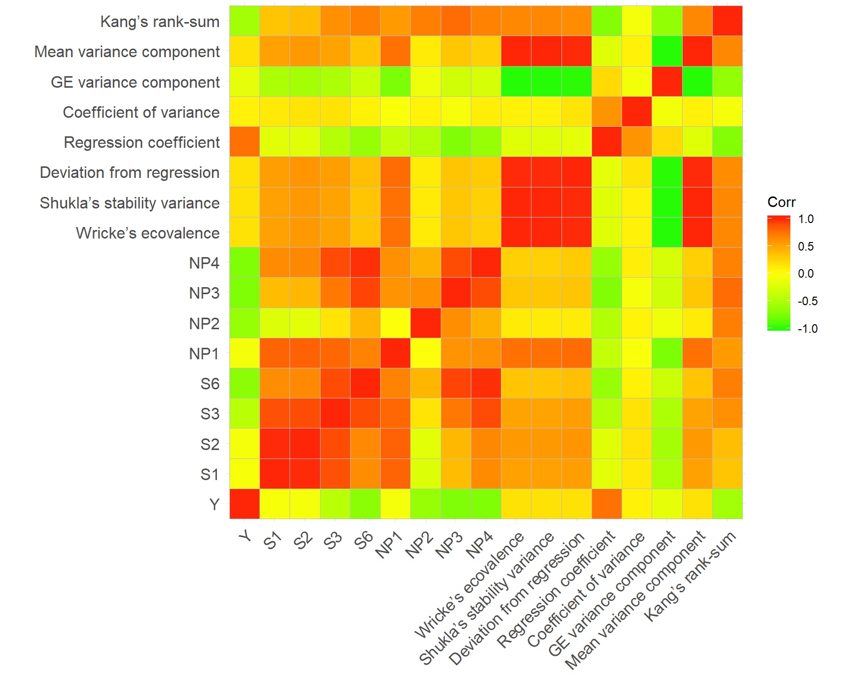
> print(results$correlation_matrix)
Y S1 S2 S3 S6 NP1 NP2 NP3 NP4 Wricke’s ecovalence Shukla’s stability variance Deviation from regression Regression coefficient Coefficient of variance GE variance component Mean variance component Kang’s rank-sum
Y 1.00000000 -0.2549881 -0.21150447 -0.4006036 -0.6289655 0.3872190 -0.09718758 -0.7620708 -0.6113699 0.13069056 0.13069056 -0.05678023 0.6724806 0.37266177 -0.13069056 0.13069056 -0.5988499
S1 -0.25498812 1.0000000 0.96587271 0.9387308 0.8182752 0.2393298 0.26387846 0.3222167 0.8400549 0.36342753 0.36342753 0.29840910 -0.2503471 -0.13787570 -0.36342753 0.36342753 0.1990615
S2 -0.21150447 0.9658727 1.00000000 0.9410083 0.7690399 0.1722324 0.34119595 0.2862215 0.7772251 0.46625079 0.46625079 0.37654936 -0.2068342 -0.09853684 -0.46625079 0.46625079 0.2530706
S3 -0.40060364 0.9387308 0.94100832 1.0000000 0.9199104 0.2230979 0.49821118 0.5394216 0.9321775 0.38576369 0.38576369 0.29455543 -0.3557948 -0.20382840 -0.38576369 0.38576369 0.4331784
S6 -0.62896553 0.8182752 0.76903989 0.9199104 1.0000000 0.1275381 0.46679096 0.7391819 0.9857845 0.20340007 0.20340007 0.25779964 -0.4362998 -0.21150745 -0.20340007 0.20340007 0.5337392
NP1 0.38721896 0.2393298 0.17223239 0.2230979 0.1275381 1.0000000 0.34567108 0.1664839 0.1850023 0.44266774 0.44266774 0.18311385 0.2069021 0.10713143 -0.44266774 0.44266774 0.2163356
NP2 -0.09718758 0.2638785 0.34119595 0.4982112 0.4667910 0.3456711 1.00000000 0.5130536 0.4759613 0.30627826 0.30627826 -0.02674715 -0.2082947 -0.20962130 -0.30627826 0.30627826 0.4759756
NP3 -0.76207085 0.3222167 0.28622150 0.5394216 0.7391819 0.1664839 0.51305356 1.0000000 0.7260324 0.14146077 0.14146077 0.17279542 -0.5234650 -0.28378894 -0.14146077 0.14146077 0.8353099
NP4 -0.61136992 0.8400549 0.77722511 0.9321775 0.9857845 0.1850023 0.47596134 0.7260324 1.0000000 0.19952002 0.19952002 0.18500493 -0.4776977 -0.27507539 -0.19952002 0.19952002 0.5094397
Wricke’s ecovalence 0.13069056 0.3634275 0.46625079 0.3857637 0.2034001 0.4426677 0.30627826 0.1414608 0.1995200 1.00000000 1.00000000 0.52370504 0.0251226 0.02182641 -1.00000000 1.00000000 0.5219578
Shukla’s stability variance 0.13069056 0.3634275 0.46625079 0.3857637 0.2034001 0.4426677 0.30627826 0.1414608 0.1995200 1.00000000 1.00000000 0.52370504 0.0251226 0.02182641 -1.00000000 1.00000000 0.5219578
Deviation from regression -0.05678023 0.2984091 0.37654936 0.2945554 0.2577996 0.1831139 -0.02674715 0.1727954 0.1850049 0.52370504 0.52370504 1.00000000 0.4403501 0.64363999 -0.52370504 0.52370504 0.4078273
Regression coefficient 0.67248064 -0.2503471 -0.20683417 -0.3557948 -0.4362998 0.2069021 -0.20829472 -0.5234650 -0.4776977 0.02512260 0.02512260 0.44035014 1.0000000 0.93333506 -0.02512260 0.02512260 -0.3630245
Coefficient of variance 0.37266177 -0.1378757 -0.09853684 -0.2038284 -0.2115075 0.1071314 -0.20962130 -0.2837889 -0.2750754 0.02182641 0.02182641 0.64363999 0.9333351 1.00000000 -0.02182641 0.02182641 -0.1447713
GE variance component -0.13069056 -0.3634275 -0.46625079 -0.3857637 -0.2034001 -0.4426677 -0.30627826 -0.1414608 -0.1995200 -1.00000000 -1.00000000 -0.52370504 -0.0251226 -0.02182641 1.00000000 -1.00000000 -0.5219578
Mean variance component 0.13069056 0.3634275 0.46625079 0.3857637 0.2034001 0.4426677 0.30627826 0.1414608 0.1995200 1.00000000 1.00000000 0.52370504 0.0251226 0.02182641 -1.00000000 1.00000000 0.5219578
Kang’s rank-sum -0.59884992 0.1990615 0.25307064 0.4331784 0.5337392 0.2163356 0.47597563 0.8353099 0.5094397 0.52195780 0.52195780 0.40782725 -0.3630245 -0.14477128 -0.52195780 0.52195780 1.0000000install.packages("ggcorrplot")library("ggcorrplot")3. Plot the heatmap for pearson's correlation matrix available in results$correlation_matrix variable
ggcorrplot(results$correlation_matrix, colors=c("#26fc06", "#ffff0a", "#ff2607"))