Giter VIP home page Giter VIP logo

cdt's Introduction

DOI View Climate Data Toolbox for MATLAB on File Exchange

Climate Data Toolbox for Matlab

CDT Contents and Documentation

Click here to view the CDT documentation online.

A version of the documentation in Chinese can be found here, translated by Shi Weiheng. 中文文档由Shi Weiheng翻译。CDT 中文翻译.pdf

Video Tutorials

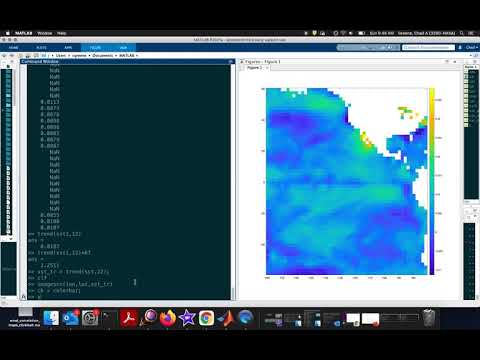
Analyzing Trends and Global Warming:

How to analyze trends in sea surface temperature using CDT

El Niño and Empirical Orthogonal Functions:

How to apply EOFs to identify ENSO

Installing the toolbox:

There are a few different ways to install this toolbox. Pick your favorite among the following:

...from the Add-On Explorer in MATLAB:

In the Home menu of MATLAB, click Add-Ons, and search for Climate Data Toolbox. Click "Add from GitHub" and that's all you need to do. Installing this way is easy and will provide the most up-to-date version available.

...or as individual files and folders:

The files in this GitHub repository will always be the most up to date. So if you want to be on the bleeding edge of innovation, get the cdt folder, put it somewhere Matlab can find it, and then right-click on it from within Matlab and select "Add to Path--Selected folder and subfolders."

...as a .mltbx toolbox:

Installing as an .mltbx is perhaps the easiest option, but I don't update the .mltbx very often, so you might not get the latest features and bug fixes.

First, download the ~100 MB .mltbx file here. After downloading the .mltbx file, installation should be as easy as double clicking on the zip file and clicking "install". Or you can navigate to it in the Matlab file explorer, right click on the .mltbx, and click "Install."

The installation process puts the files in a folder called something like:

~MATLAB/Add-Ons/Toolboxes/Climate Data Toolbox/

If that's not correct, find the CDT folder by typing this into the Matlab Command Window:

which cdt -all

If the which hunt still turns up nothing, that suggests the toolbox hasn't been properly installed.

After installation:

Type

cdt

into the command line to check out the documentation.

Citing CDT:

Please cite our paper!

Chad A. Greene, Kaustubh Thirumalai, Kelly A. Kearney, José Miguel Delgado, Wolfgang Schwanghart, Natalie S. Wolfenbarger, Kristen M. Thyng, David E. Gwyther, Alex S. Gardner, and Donald D. Blankenship (2019). The Climate Data Toolbox for MATLAB. Geochemistry, Geophysics, Geosystems, 20, 3774-3781. doi:10.1029/2019GC008392

The Climate Data Toolbox is also mirrored on the MathWorks File Exchange site here.

cdt's People

Contributors

chadagreene avatar jonlighthall avatar kakearney avatar kakearney-noaa avatar mheberger avatar

Stargazers

 avatar  avatar  avatar  avatar  avatar  avatar  avatar  avatar  avatar  avatar  avatar  avatar  avatar  avatar  avatar  avatar  avatar  avatar  avatar  avatar  avatar  avatar  avatar  avatar  avatar  avatar  avatar  avatar  avatar  avatar  avatar  avatar  avatar  avatar  avatar  avatar  avatar  avatar  avatar  avatar  avatar  avatar  avatar  avatar  avatar  avatar  avatar  avatar  avatar  avatar  avatar  avatar  avatar  avatar  avatar  avatar  avatar  avatar  avatar  avatar  avatar  avatar  avatar  avatar  avatar  avatar  avatar  avatar  avatar  avatar  avatar  avatar  avatar  avatar  avatar  avatar  avatar  avatar  avatar  avatar  avatar  avatar  avatar  avatar  avatar  avatar  avatar  avatar  avatar  avatar  avatar  avatar  avatar  avatar  avatar  avatar  avatar  avatar  avatar  avatar

Watchers

 avatar  avatar  avatar  avatar  avatar  avatar  avatar  avatar  avatar  avatar  avatar  avatar  avatar  avatar  avatar  avatar  avatar  avatar  avatar

cdt's Issues

Redundant mean removal in nao index computation

In the function nao, the mean is removed in lines 64 through 66. However, the mean is already removed by the standardize call in lines 60 through 62, which makes the second removal redundant.

time step returned by the SPEI

SPEI returns a time step equal to the input variable integrationtime. Although not wrong, that does not agree with the spirit of SPEI. The time step of the returned SPEI time-series should be the same as the meteorological time-series that goes as input. The integration should then occur as a sliding window.

Landmass avoidance using island

Hi Chad,

I am writing a navigating code for a vessel in seaway, and one of the requirements is to check if the next coordinate is land or sea. If I know a set of coordinates of subsea constructions, oil rigs, etc. How can I add these polygon area into the island function.

Thank you for your time and concern reading my question,

Sicnerely,

implementing SPI

User Behzad Navidi asked if implementing SPI would require significant additional changes to the code.

Answer:

Computing the SPI will only require a small
change in the code. The water balance D=P-E will no longer be necessary
and can be replaced with D=P. This would mean that the standardization
of the variable later could be made with the gamma function, but I
don't see a reason why the currently implemented log-logistic won't work.

That would require creating a new function spi.m that would be similar
to spei.m only with the small change described above. Definitely worth
doing.

Add variable baseline functionality to anomaly plot function

The anomaly plot function could be much more versatile by allowing the user to specify a variable baseline. This is useful for visualising differences between the annual trend of a given parameter and its climatological mean. This is an example plot:
example

Implementing this into the code is pretty straightforward:

  1. Line 81

Assert that the base is either a scalar (constant baseline) or a vector the same length as x and y (variable baseline):

assert(isscalar(base) | numel(base)==numel(y),'Input error: Base value must be a scalar or a vector of the same length as x and y.')
  1. Data Manipulation section (line 103)

If base is a scalar, convert it into a column vector the length of y (before "Columnate inputs to ensure...":

% If base is a scalar convert it into a column vector the length of y:
if isscalar(base)
    base = repmat(base,numel(y),1);
end

Columnate base just like x and y (only relevant if base is not a scalar):

base = base(:);

Find NaNs both in y and base so filling will work (and remove them from base as well):

% If y or base contains nans, ignore them so filling will work:
ind = (isfinite(y) & isfinite(base));
...
base = base(ind);

The intersections subfunction now simplifies as follows:

[xc,yc] = intersections(x,y,x,base);

Add zero crossings to base:

% Add zero crossings to the input dataset and sort them into the proper order: 
...
base = [base;yc];
...
base = base(ind);

Splitting the data into a top and bottom dataset changes as follows:

% Start thinking about this as two separate datasets which share baseline values where they meet: 
ytop = y; 
ytop(ytop<base) = base(ytop<base); 
ybot = y; 
ybot(ybot>base) = base(ybot>base); 
  1. Plotting

Instead of using area we now need to use fill, the output remains the same:

% Plot the top half: 
htop = fill([x;flipud(x)],[ytop;flipud(base)],topcolor);

% Plot the bottom half: 
hbot = fill([x;flipud(x)],[ybot;flipud(base)],bottomcolor);

VOILA! This will allow the user to provide either a constant or a variable baseline and the code will do the rest:
example2

Here is a copy of the adjusted code:
anomaly_JW.m.zip

I hope this is helpful.

Cheers,
Jake

The Z-value in the mann_kendall.m is incorrect when S>=0

ind = S>=0;
Line 121: Z(ind) = ((S(ind)-1)/StdS).(S(ind));
should be: Z(ind) = ((S(ind)-1)/StdS).
(S~=0);

The (S(ind)) is only correct when ind = logical 0. When ind = logical 1, Z(ind) = ((S(ind)-1)/StdS).*(S(ind)) = ((S(ind)-1)/StdS).*S. This is incorrect.

A Chinese version of CDT Contents

CDT 中文翻译.pdf
I'm using CDT and I'm exciting about finding such a terrific toolbox for processing meteorology data. However as I'm a Chinese, some of my colleagues or classmates cannot understand the wiki and instruction exactly. So I translate the CDT Contents (mostly from https://www.chadagreene.com/CDT/CDT_Contents.html ) into Chinese.
The work has been started about 5 months ago. Due to my personal reasons, I feel very ashamed of delaying the process of translation. Last week, I translated and typeset all the function documents of the toolbox, which took a long time longer than expected. This is the PDF version after typesetting. I'm not sure if there will be any errors in it. Please review it if convenient.
I hope it may help other people when using this toolbox.

CDT documenation is not searchable in matlab.

Starting in R2022a, the builddocsearchdb function creates the subfolder helpsearch-v4 to contain the search database files. Previously, builddocsearchdb created a subfolder named helpsearch-v3. As a Result the CDT Documentation is not searchable in Matlab R2022a or later
image.

Incorrect masks generated for specific cases of 2Drange

If coordinates on a 0 to 360 grid cross 180 then the resulting mask will nearly be the inverse of the intended mask. The reason for this is because of the combination of changing to a -180 to 180 coordinate system and the assumption that the smaller longitude is the leftmost and larger rightmost (lines referenced below).

CDT/cdt/geomask.m

Lines 95 to 99 in 8838903

ind = lon>180;
lon(ind) = lon(ind)-360;
indv = lonv>180;
lonv(indv) = lonv(indv)-360;

mask = lat>min(latv) & lat<max(latv) & lon>min(lonv) & lon<max(lonv);

EX (simplified to 1d):
lon = [0 60 120 180 240 300];
lonv = [100 250];

the expected mask is
[0 0 1 1 0 0]

both inputs would be changed to -180 to 180 coordinate system
lon = [0 60 120 180 -120 -60];
lonv = [100 -110];

min(lonv) is now -110 instead of 100 and lon>min(lonv) would produce
[1 1 1 1 0 1]
and lon<max(lonv) would produce
[1 1 0 0 1 1]
the logical and of these 2 produces
[1 1 0 0 0 1]

I propose assuming the first value of lonv is the leftmost input. This would be more in line with how someone would read the value and find it on a globe.

if lonv(1) > lonv(2)
mask = lat>min(latv) & lat<max(latv) & (lon>lonv(1) | lon<lonv(2));
else
mask = lat>min(latv) & lat<max(latv) & (lon>lonv(1) & lon<lonv(2));
end

Regarding basics - Raw/Processed i/ps??

Hello Chad Greene,
I'm not sure if this page is still active and if you're responding to the queries.
But, I have a few basic related issues:

  1. do we need to use raw data in eofs? or use the preprocessed data?
    I asked for raw data - assuming, the EOF function does preprocess the data provided.
  2. I anyway used detrended and de-seasonal data - but the resultant is close to zero - so, I wonder if the function accepts such i/ps?
    When I used de-seasonal data: I get the following error
    image

My inputs are 3*3 matrix: 161 321 66: 66 is the time component !!! (seasonal data - 3 months for 22 years).
Can the team please help me correct this?

Geomask error for polygons

Hi,
I'm new to CDT and new to GitHub. I am trying to write my thesis on climate change with the help of Matlab and CDT…
And I found out that the geomask does not work well when entering multiple countries = polygons (at least according to the instructions).

Therefore, instead of the part in the geomask.m function:

indv = lonv > 180;
lonv(indv) = lonv(indv) - 360;

I suggest using:

% The following part of the code (lonv correction) was made by Tomáš Poláček
% Check if lonv is of type cell
if iscell(lonv)
    % Iterate over individual rows
    for i = 1:numel(lonv)
        % If the given line contains double data
        if isnumeric(lonv{i})
            indv = lonv{i} > 180;
            lonv{i}(indv) = lonv{i}(indv) - 360;
        end
    end
else
    % If lonv is not of cell type, it is a different variable type,
    % we perform the operation on the entire lonv (if it is of type double)
    if isnumeric(lonv)
        indv = lonv > 180;
        lonv(indv) = lonv(indv) - 360;
    end
end

There is also inaccuracy in CDT help (geomask):
% For this sample 1 degree resolution grid:
[Lat,Lon] = geogrid;

(geogrid is not defined function)

So maybe it will be better to use something like:
[Lon,Lat] = meshgrid(lon, lat);

Thank you in advance for your response and possible correction of my statement.

distance2coast.mat do not coast at some locations (around 18 deg E and 15 deg N).

The distance2coast.mat file contains the distance of 1/8 degree grid over ocean from the coast. But at the above mentioned location it do not follow. The distance2coast.mat data is verified with load coast data and Etopo2 data. In both the cases it do not follow.

Known issues i noted while creating this issue:
"this function is probably best suited for mesoscale processes that aren't affected by little islands." (Source: https://chadagreene.com/CDT/dist2coast_documentation.html)

Add daily_insolation.m functionality to handle Berger 1978 solution

The current version of daily_insolation.m in the CDT calculates the orbital parameters from the BER90 solution described in Berger & Loutre 1991. As noted in Berger & Loutre 1991 (see conclusion bullet point no. 4) the BER78 solution "is preferable to BER90 for the last glacial-interglacial cycles because of its better accuracy close to present-day times". This is most easily checked by comparing the eccentricity value from daily_insolation.m (0.0172571) for 2000CE, compared to Wikipedia (0.0167086), a difference of 0.5485e-3. Using the BER78 solution eccentricity = 0.0167441, a difference of 0.0355e-3 (compared to Wikipedia) and an extra degree of precision. A similar improvement is found in the longitude of perihelion for 2000CE, Wikipedia = 102.9, daily_insolation.m = 100.51, and BER78 = 101.18.

I therefore propose the attached solution (daily_insolation_new.zip) which requires the mat file Berger.zip. This new function allows the user to pass in an option handle 'BER78' which calculates the eccentricity, obliquity, and longitude of perihelion from the BER78 solution described in Berger & Loutre 1991.

Description of changes
I have updated the comments under 'syntax' and 'description' to describe the new functionality.

The updates to the code are:

  1. line 80 to handle the case of multiple options, i.e. 'constant',value, 'mjmd', and 'BER78'.
    narginchk(3,8)

  2. lines 107-111 to handle the new option

if any(strcmpi(varargin,'BER78'))
    BER78 = true; % calculate orbital parameters from Berger 1978
else
    BER78 = false;
end
  1. lines 116-120 to select the orbital parameters function depending on the option
if BER78
    [ecc,epsilon,omega]=orbital_parameters_BER78(kyear); % function is below in this file
else
    [ecc,epsilon,omega]=orbital_parameters(kyear); % function is below in this file
end
  1. lines 190-236 the new orbital parameters function
% === Calculate orbital parameters from Berger 78 ===
% as described in Berger & Loutre 1991
function [ecc,epsilon,omega] = orbital_parameters_BER78(kyear)
t=-kyear.*1000; % convert kyr to yr and flip sign

% Load the tables from Berger & Loutre 1991
load('Berger.mat','Berger');
Table1 = Berger.Berger78.Table1;
Table4 = Berger.Berger78.Table4;
Table5 = Berger.Berger78.Table5;

% Constants from Table 9 in Berger & Loutre 1991
psibar = 50.439273/60./60. * pi/180 ;   % kbar
estar  = 23.320556;                     % eps *
zeta   = 3.392506 * pi/180;             % alpha

twopi  = 2*pi;
sectorad = pi/(180*60.*60);

% Order of table columns 'Term','Amp','Rate','Phase','Period'
M   = Table4(:,2);            % Amp
g   = Table4(:,3).*sectorad;  % Rate
b   = Table4(:,4).*pi./180;   % Phase
F   = Table5(:,2).*sectorad;  % Amp
fp  = Table5(:,3).*sectorad;  % Rate
d   = Table5(:,4).*pi./180;   % Phase
A   = Table1(:,2)./60./60;    % Amp
f   = Table1(:,3).*sectorad;  % Rate
phi = Table1(:,4).*pi./180;   % Rate


eps = estar + sum(A.*cos(f.*t+phi));

esinpi = sum(M.*sin(g.*t+b));
ecospi = sum(M.*cos(g.*t+b));
psi    = psibar.*t + zeta + sum(F.*sin(fp.*t +d));

e = sqrt(esinpi.^2+ecospi.^2);
Pi = atan(esinpi./ecospi)+pi.*(ecospi<0);
eps = eps * pi./180;
varpi = mod(Pi+psi+pi,twopi);

epsilon=eps;
ecc=e;
omega=varpi;

end

In addition to the above, it would not be too difficult to calculate the BER90 solution in the same way as the BER78 method
orbital_parameters_BER90.zip.

I hope you find this useful.
Andrew

MLD calculation mismatch

Appreciate your work! It's a useful toolbox!
In mld.m profile, IN-SITU temperature is inputted. However, to calculate potential density, the code refers to gsw_rho, in which the input arguments are CONSERVATIVE temperature (or potential temperature) and ABSOLUTE SALINITY (g/kg). The unit of salinity is not illustrated in the header lines. The difference in the type of temperature and an uncommon salinity unit could lead to a serious mistake. Simply change gsw_rho to sw_pden would do the trick. :p
ps: There's a typo on https://www.chadagreene.com/CDT/mld_documentation.html. The examples adopt a T threshold of 0.2 deg C, yet it's changed to 0.02 deg in the code below.

Recommend Projects

  • React photo React

    A declarative, efficient, and flexible JavaScript library for building user interfaces.

  • Vue.js photo Vue.js

    🖖 Vue.js is a progressive, incrementally-adoptable JavaScript framework for building UI on the web.

  • Typescript photo Typescript

    TypeScript is a superset of JavaScript that compiles to clean JavaScript output.

  • TensorFlow photo TensorFlow

    An Open Source Machine Learning Framework for Everyone

  • Django photo Django

    The Web framework for perfectionists with deadlines.

  • D3 photo D3

    Bring data to life with SVG, Canvas and HTML. 📊📈🎉

Recommend Topics

  • javascript

    JavaScript (JS) is a lightweight interpreted programming language with first-class functions.

  • web

    Some thing interesting about web. New door for the world.

  • server

    A server is a program made to process requests and deliver data to clients.

  • Machine learning

    Machine learning is a way of modeling and interpreting data that allows a piece of software to respond intelligently.

  • Game

    Some thing interesting about game, make everyone happy.

Recommend Org

  • Facebook photo Facebook

    We are working to build community through open source technology. NB: members must have two-factor auth.

  • Microsoft photo Microsoft

    Open source projects and samples from Microsoft.

  • Google photo Google

    Google ❤️ Open Source for everyone.

  • D3 photo D3

    Data-Driven Documents codes.